Numerical Calculus I: differentiation
December 2025
Outline
- Introduction
- Finite differencing
- Automatic differentiation
- Recap
Introduction
Introduction
Statistical computations often involve computing derivatives and integrals.
For theoretical work, we often analyze these objects purely mathematically.
For practical work, we need to actually differentiate and integrate specific functions.
In many cases, this can be done exactly but there are many situations where we need to approximate a derivative / integral.
In some situations we really want an algorithmic solution as a fitting procedure may involve
creating new functions, and
doing some calculus with them.
Finite differencing
Derivatives
The derivative of a function \(f:\mathbb{R}\to\mathbb{R}\) is the function \(f'\) given by \[f'(x)=\lim_{h\to0}\frac{f(x+h)-f(x)}{h},\] if the limit exists.
Symbolic computations (e.g. in Maple) can compute lots of derivatives, but we are interested here in a different approach.
Natural approach: \[f'_{h}(x)=\frac{f(x+h)-f(x)}{h},\] with \(h\) “suitably small”.
Gradients and partial derivatives
The \(i\)th partial derivative of \(f:\mathbb{R}^{d}\to\mathbb{R}\) at \({\bf a}\) is \[\frac{\partial f}{\partial x_{i}}({\bf a})=\lim_{h\to0}\frac{f(a_{1},\ldots,a_{i-1},a_{i}+h,a_{i+1},\ldots,a_{d})-f({\bf a})}{h}.\]
The gradient of a function \(f:\mathbb{R}^{d}\to\mathbb{R}\) is the vector of partial derivatives \[\left(\frac{\partial f}{\partial x_{1}},\ldots,\frac{\partial f}{\partial x_{d}}\right).\]
These are used a lot and \(d\) can be very large indeed.
We “only” need to approximate derivatives of \(f:\mathbb{R}\to\mathbb{R}\).
Cancellation error
One problem: computers don’t do precise calculations.
They use a large number of real numbers to approximate the whole of \(\mathbb{R}\).
This is annoying! Consider the code in the lecture notes:
a <- 1e16; b <- 1e16 + pi; d <- b-a
The value of
dafter these operations is 4, which is quite far from \(\pi\).Example of a problem: taking the difference of two floating point numbers with similar size and sign.
- Exactly the kind of issue we have with approximating \(f'_{h}(x)\).
Approximation error: part I
Consider Taylor’s Theorem: \[f(x+h)=f(x)+hf'(x)+\frac{1}{2}h^{2}f''(\xi),\] for some \(\xi\in(x,x+h)\).
Assume \(|f''|\leq L\) everywhere, at least to make a point.
Rearranging gives \[\left|\frac{f(x+h)-f(x)}{h}-f'(x)\right|=\frac{1}{2}h|f''(\xi)|\leq\frac{Lh}{2}.\]
Quantifies the error from taking finite \(h\).
Approximation error: part II
We can’t compute \(f\) pointwise exactly.
Suppose we actually compute \(\tilde{f}\), which satisfies the relative error criterion: \[|\tilde{f}(x)-f(x)|\leq\epsilon|f(x)|.\]
Then if \(|f(z)|\leq L_{f}\) everywhere, we obtain \[\left|\frac{\tilde{f}(x+h)-\tilde{f}(x)}{h}-\frac{f(x+h)-f(x)}{h}\right|\leq2\frac{\epsilon L_{f}}{h}.\]
So we have bounded the difference between what we compute and \(f'_{h}(x)\).
Approximation error: the tradeoff
Now we can bound the total error (triangle inequality): \[\left|\frac{\tilde{f}(x+h)-\tilde{f}(x)}{h}-f'(x)\right|\leq\frac{Lh}{2}+\frac{2\epsilon L_{f}}{h}.\]
Minimizing w.r.t. \(h\) gives \[h=\sqrt{\frac{4\epsilon L_{f}}{L}},\] which manages the tradeoff between the “rounding error” and not taking the limit.
This explains why \(h\sim O(\sqrt{\epsilon})\) is relatively widespread in practice.
Choosing the finite-difference interval
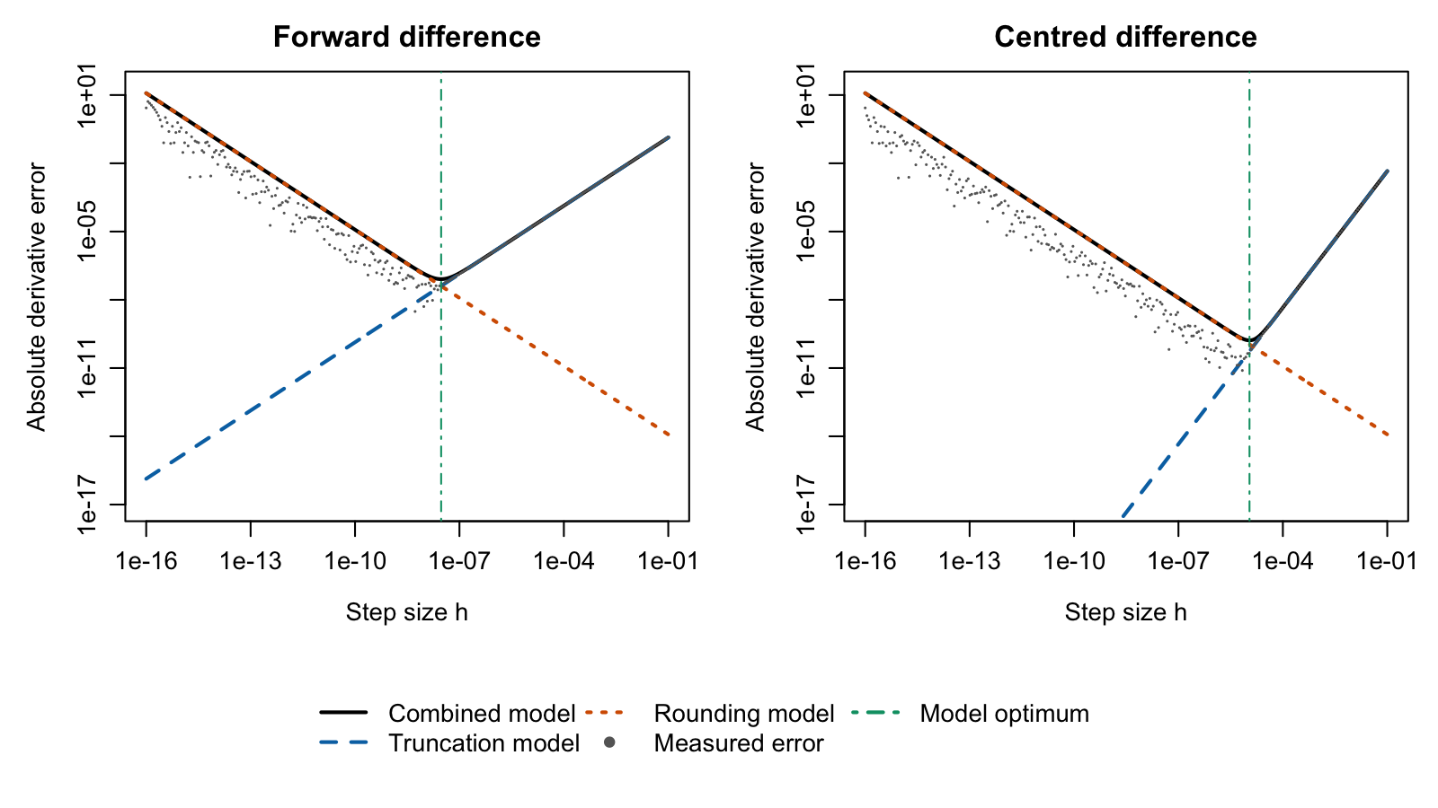
For \(f(x)=e^x\) at \(x=1\): dots are measured floating-point errors; curves are leading-order error models, rather than strict bounds. Green lines mark the model minima.
Other finite difference formulae
There are other schemes, e.g \[f'_{h}(x)=\frac{f(x+h)-f(x-h)}{2h},\] which can be more accurate.
Similarly, there are formulae for approximating higher order derivatives: \[f''_{h}(x)=\frac{f(x+h)-2f(x)+f(x-h)}{h^{2}}.\]
These can essentially be analyzed the same way.
Automatic differentiation
Differentiation is “easy”
Computations can be expressed as compositions of functions involving elementary arithmetic operations.
In principle, the chain rule and some “primitive” derivatives are sufficient to allow computation of any derivative.
- This is very different to integration.
So we could automate it!
Symbolic computation is one route, but this tends to lead to complicated expressions quite quickly.
Here, we will look at automatic differentiation, a quite different approach.
Automatic differentiation
Goal: compute derivatives up to floating-point error as a by-product of using the computer code that evaluates the function.
Idea: use the chain rule.
First the univariate case, for simplicity.
If \(y=f_{3}\circ f_{2}\circ f_{1}(x)\), then write \[w_{0}=x\quad,w_{1}=f_{1}(x),\quad w_{2}=f_{2}(w_{1}),\quad y=w_{3}=f_{3}(w_{2}).\]
We obtain \[\frac{\partial y}{\partial x}=\frac{\partial y}{\partial w_{2}}\frac{\partial w_{2}}{\partial w_{1}}\frac{\partial w_{1}}{\partial x}=\frac{\partial f_{3}}{\partial w_{2}}(w_{2})\frac{\partial f_{2}}{\partial w_{1}}(w_{1})\frac{\partial f_{1}}{\partial x}(x).\]
Can compute each partial derivative \[\frac{\partial f_{i}}{\partial w_{i-1}}(w_{i-1})\] when computing \(w_{i}=f_{i}(w_{i-1})\), and then take the product of these (accumulate).
Automatic differentiation: forward mode
Now with vectors; assume \(f:\mathbb{R}^{n}\to\mathbb{R}^{m}\).
One can lay out the vectors so that \[{\bf w}_{i}=f_{i}({\bf w}_{i-1}),\] with \({\bf x}={\bf w}_{0}\), \(f_{i}:\mathbb{R}^{d_{i-1}}\to\mathbb{R}^{d_{i}}\), \({\bf w}_{i}\in\mathbb{R}^{d_{i}}\) and \({\bf y}={\bf w}_{L}\).
Wolog assume we want the partial derivative of \(y\) w.r.t. \(x_{1}\).
We compute everything forwards: as we compute \(w_{ij}\) we also compute \[\frac{\partial w_{ij}}{\partial x_{1}}=\sum_{k=1}^{d_{i-1}}\frac{\partial w_{ij}}{\partial w_{i-1,k}}\frac{\partial w_{i-1,k}}{\partial x_{1}}.\]
Forward mode example
Consider \(y=\exp(x_{1}x_{2})+x_{1}^{2}\), evaluated at \({\bf x}=(a,b)\).
Write \({\bf w}_{0}=(x_{1},x_{2})\), \({\bf w}_{1}=(w_{01}\cdot w_{02},w_{01}\cdot w_{01})\), \({\bf w}_{2}=(\exp(w_{11}),w_{12})\) and \(y=w_{3}=w_{21}+w_{22}\).
Find \({\bf w}_{0}=(a,b)\) \[\left(\frac{\partial w_{01}}{\partial x_{1}},\frac{\partial w_{02}}{\partial x_{1}}\right)=(1,0).\] Then \({\bf w}_{1}=(ab,a^{2})\) and \[\begin{align*} \frac{\partial w_{11}}{\partial x_{1}} & =\frac{\partial w_{11}}{\partial w_{01}}\frac{\partial w_{01}}{\partial x_{1}}+\frac{\partial w_{11}}{\partial w_{02}}\frac{\partial w_{02}}{\partial x_{1}}\\ & =w_{02}\cdot1+w_{01}\cdot0=b. \end{align*}\] Similarly, \[\begin{align*} \frac{\partial w_{12}}{\partial x_{1}} & =\frac{\partial w_{12}}{\partial w_{01}}\frac{\partial w_{01}}{\partial x_{1}}+\frac{\partial w_{12}}{\partial w_{02}}\frac{\partial w_{02}}{\partial x_{1}}\\ & =2a\cdot1+0\cdot0=2a. \end{align*}\]
Forward mode example
Consider \(y=\exp(x_{1}x_{2})+x_{1}^{2}\), evaluated at \({\bf x}=(a,b)\).
Write \({\bf w}_{0}=(x_{1},x_{2})\), \({\bf w}_{1}=(w_{01}\cdot w_{02},w_{01}\cdot w_{01})\), \({\bf w}_{2}=(\exp(w_{11}),w_{12})\) and \(y=w_{3}=w_{21}+w_{22}\).
Now, \({\bf w}_{2}=(\exp(ab),a^{2})\) \[\begin{align*} \frac{\partial w_{21}}{\partial x_{1}} & =\frac{\partial w_{21}}{\partial w_{11}}\frac{\partial w_{11}}{\partial x_{1}}+\frac{\partial w_{21}}{\partial w_{12}}\frac{\partial w_{12}}{\partial x_{1}}\\ & =\exp(w_{11})\cdot b+0\cdot2a=\exp(ab)\cdot b, \end{align*}\] and \[\begin{align*} \frac{\partial w_{22}}{\partial x_{1}} & =\frac{\partial w_{22}}{\partial w_{11}}\frac{\partial w_{11}}{\partial x_{1}}+\frac{\partial w_{22}}{\partial w_{12}}\frac{\partial w_{12}}{\partial x_{1}}\\ & =0\cdot b+1\cdot2a=2a \end{align*}\]
Finally \(w_{3}=\exp(ab)+a^{2}\) and \[\frac{\partial w_{3}}{\partial x_{1}}=1\cdot\exp(ab)\cdot b+1\cdot2a.\]
Forward mode: a computational graph
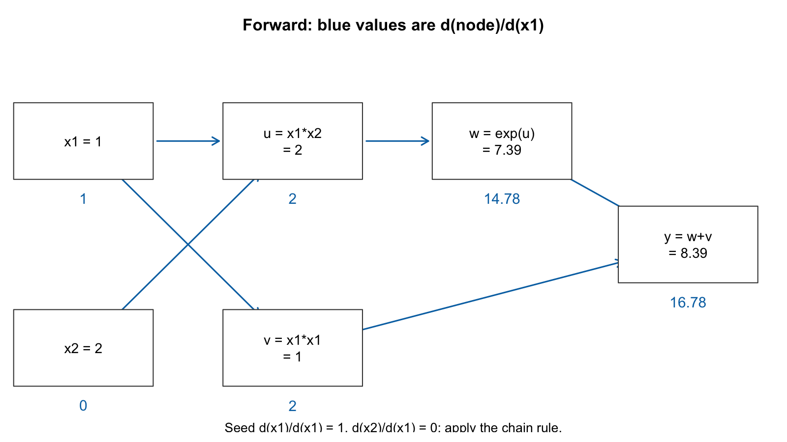
The worked example at \((a,b)=(1,2)\).
Forward mode recap
We’ve looked at the computation of \(\partial y/\partial x_{1}\) at a particular point.
You can get, e.g., \(\partial y/\partial x_{2}\) by running another pass, or computing relevant quantities alongside.
Implicitly, we are applying the chain rule for Jacobians \[J_{h}({\bf x})=\left[\begin{array}{ccc} \frac{\partial h_{1}({\bf x})}{\partial x_{1}} & \cdots & \frac{\partial h_{1}({\bf x})}{\partial x_{n}}\\ \vdots & \ddots & \vdots\\ \frac{\partial h_{m}({\bf x})}{\partial x_{1}} & \cdots & \frac{\partial h_{m}({\bf x})}{\partial x_{n}} \end{array}\right],\] i.e. using the identity \[J_{g\circ f}({\bf x})=J_{g}(f({\bf x}))J_{f}({\bf x}).\]
Of course, part of the issue is how to compute these things automatically:
- source code transformation / operator overloading.
Reverse mode
An alternative to forward mode is reverse mode.
We can use associativity of matrix multiplication to justify computing the other way around.
To be concrete, assume \({\bf y}=g({\bf x})=f_{3}\circ f_{2}\circ f_{1}({\bf x})\), with \(f_{1}:\mathbb{R}^{n}\to\mathbb{R}^{p}\), \(f_{2}:\mathbb{R}^{p}\to\mathbb{R}^{q}\), \(f_{3}:\mathbb{R}^{q}\to\mathbb{R}^{m}\).
Chain rule: \[J_{g}({\bf x})=J_{f_{3}}(f_{2}\circ f_{1}({\bf x}))J_{f_{2}}(f_{1}({\bf x}))J_{f_{1}}({\bf x}),\] which is a product of \(3\) matrices of size \(m\times q\), \(q\times p\) and \(p\times n\).
Forward complexity (right to left): \(qpn+mqn\).
Reverse complexity (left to right): \(mqp+mpn\).
Simple case, \(m=1\) and \(p=q=n\). Then forward is \(\mathcal{O}(n^{3})\) but reverse is \(\mathcal{O}(n^{2})\).
Reverse mode: the same graph
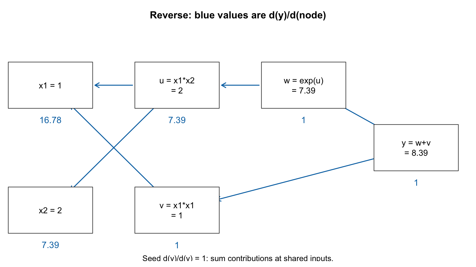
One backward sweep gives derivatives with respect to both inputs.
Reverse mode: memory / optimal computation
In forward mode, we only need one “layer” to compute the next layer.
A naive reverse-mode implementation stores values and local derivatives for its backward sweep.
This can have a large memory cost; checkpointing trades recomputation for storage.
Matrix-level differentiation can avoid recording every scalar operation. One can also mix forward and reverse mode.
- Any sequence of appropriate matrix multiplications is fine.
The optimal sequence is NP-hard (strange examples) or at least of open complexity.
A caveat
Consider the function, for positive \(y\), \[B(y;\lambda)=\left\{ \begin{array}{ll} (y^{\lambda}-1)/\lambda & \lambda\ne0\\ \log(y) & \lambda=0 \end{array}\right..\]
If \(f(\lambda)=y^{\lambda}=\exp(\log y\cdot\lambda)\), we have \(f^{(k)}(\lambda)=\log(y)^{k}y^{\lambda}\).
Using this, we can find that \[\lim_{h\to0}\frac{y^{h}-1}{h}=\log(y),\] and \[\frac{\partial B}{\partial\lambda}(y;0)=\lim_{h\to0}\frac{\frac{y^{h}-1}{h}-\log(y)}{h}=\frac{1}{2}\log(y)^{2},\] but AD will not obtain this expression using only the evaluation of \(B(y;0)\).
Recap
Wrapping up
Finite differences are a classical and fairly robust way to approximate derivatives of sufficiently smooth functions.
You get approximate values, trading off two sources of error.
No problem if computation of function involves conditional statements!
Symbolic computation (e.g. in Maple or Mathematica) can also be useful.
- You get exact expressions, useful mainly for simple enough functions.
Automatic differentiation applies the chain rule to the executed computation.
- Derivative values are accurate up to floating-point error.