Some other topics
December 2025
Outline
- Introduction
- Pseudorandom number generation
- Sparse matrices
- Parallel computing
- Random algorithms
- Recap
Introduction
Introduction
A few topics today:
Pseudorandom number generators
Sparse matrices
Parallel computing
Random algorithms
Pseudorandom number generation
Pseudorandom number generation (PRNG)
Computers typically use PRNGs in algorithms.
They can produce new “seemingly” random numbers much faster than external “truly” random sources.
Old PRNGs are usually too simple.
- E.g., the linear congruential generators described in the notes.
Things that matter: the period (samples before repeating) and the quality.
There are software packages that “test” whether random numbers pass tests.
- Can be thought of as hypothesis tests with \(H_{0}\) being that the numbers are i.i.d.
PRNGs: recent activity
Until recently, the Mersenne Twister algorithm was very popular and has a huge period of \(2^{19937}-1\).
There has recently been a flurry of activity.
Counter-based PRNGs (cryptographic-inspired).
PCG Family: permuted congruential generators.
xoshiro / xoroshiro.
Lots more!
Different PRNGs have different apparent strengths, including speed.
For parallel computing, useful to have skip-ahead functionality, or allocate each thread a different block of a large orbit.
Sparse matrices
Sparse matrix computations
Many statistical computations involve matrices which contain very high proportions of zeroes: these are sparse matrices.
Numerical linear algebra: most computations are additions, subtractions and multiplications of pairs of numbers.
There is no point doing the computations involving \(0\): answer is known in advance.
There is also no point storing the whole matrix; just store the non-zero values and their locations.
Example in notes: a design matrix combining two categorical variables. Most entries are \(0\).
Special routines for manipulating sparse matrices, e.g. decompositions that preserve sparsity.
An example
Consider a simple problem that helped create a big company.
![]()
The Google search homepage in 1998

Ranking webpages
Ranking based on the average occupation time of each webpage for a random web surfer...
with probability \(\alpha\) follows links uniformly at random on the page they are on?
- on a page with no links, sample a page from a fixed distribution.
- with probability \(1-\alpha\) samples a page from a given (possibly personal) distribution.
The internet (some of it, anyway)
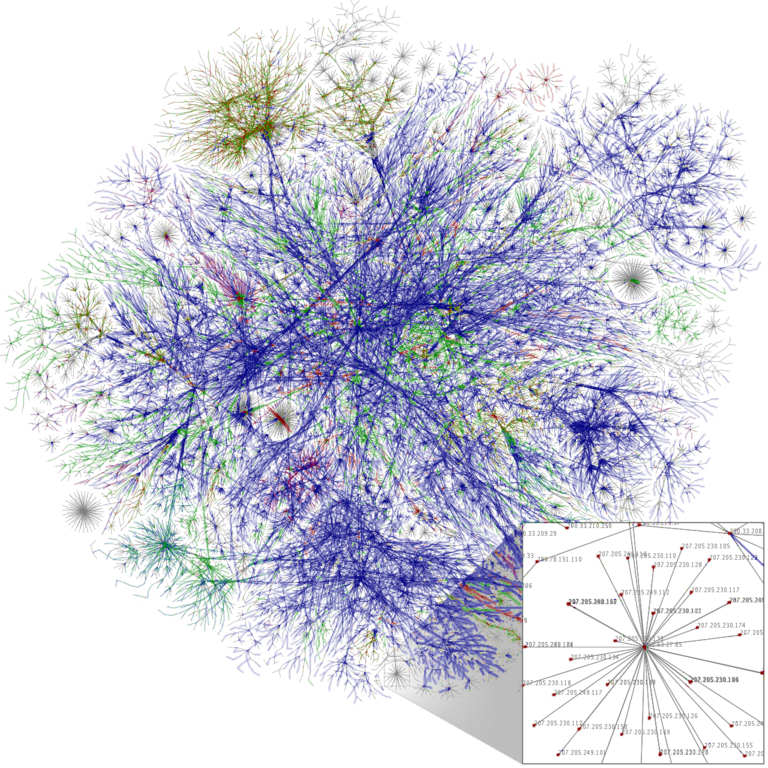
Source: Wikimedia Commons
A stochastic matrix
The relevant data is the \(n\times n\) (directed) adjacency matrix \(A\).
\(A\) is a matrix of all zeros, except \(A_{ij}=1\) if there is a link from page \(i\) to page \(j\).
No self-links and \(A\) is a very sparse matrix.
From this we create a substochastic matrix \(H\) via \[H_{ij}=\frac{A_{ij}}{\sum_{k=1}^{n}A_{ik}},\] if the denominator is positive and \(H_{ij}=0\) otherwise.
A stochastic matrix \(S\) is then defined via \[S=H+dw^{T},\] where \(d\) is a binary vector with \(d_{i}=1\) if and only if \(\sum_{k=1}^{n}A_{ik}=0\), and \(w\) is some simple distribution.
Random surfer stochastic matrix
\(S\) is the transition matrix of the random surfer who just chooses links uniformly at random.
Now we add the possibility of choosing from a “personalization” distribution. Set \[G=\alpha S+(1-\alpha){\bf 1}p^{T},\] where \(p\) is the personalization distribution, with\(0\leq\alpha<1\) and \(p_{i}>0\) for all \(i\).
\(A\) and hence \(H\) are sparse. But \(S\) can have dense dangling-node rows, and \(G\) is dense.
To compute average occupation time, use PerronFrobenius for finite Markov chains: \[\mu^{T}G^{m}\to\pi^{T},\] where \(\mu\) is an arbitrary probability distribution and \(\pi\) is the (unique) stationary distribution given our assumptions.
So we want to compute \(\mu^{T}G^{m}\) for large \(m\).
Sparsity before and after teleportation
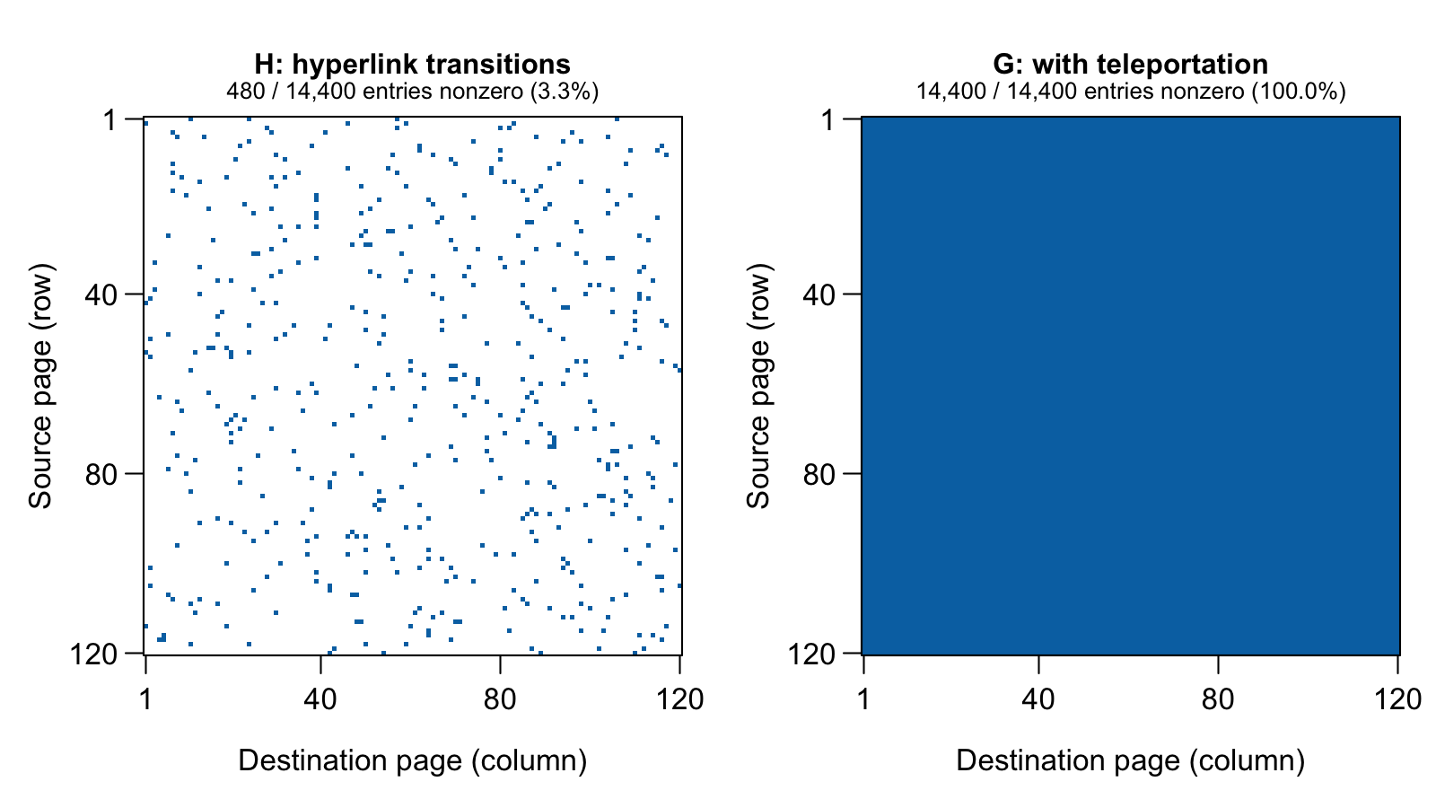
Blue cells are nonzero; white cells are zero. Each of the 120 pages has four outlinks. With \(\alpha=0.85\) and uniform teleportation, every entry of \(G\) is positive.
Storage for a large network
1 million pages, averaging 10 outlinks per page: 10 million links.
| Matrix | Explicit representation | Storage |
|---|---|---|
| \(H\) | Compressed sparse columns | 124 MB |
| \(G\) | Dense, \(10^{12}\) entries | 8,000 GB (8 TB) |
- Double-precision values: 8 bytes each. Sparse indices and column pointers: 4 bytes each.
- \(H\): \(12\times10^7 + 4\times(10^6+1)\) bytes; \(G\): \(8\times(10^6)^2\) bytes.
- Decimal units; array storage only, excluding object overhead and working memory.
Store \(H\) and vectors; apply \(G\) through its formula.
Sparse power iteration
How can we do this without ever constructing \(G\)? Use \[\begin{align*} \nu^{T}G & =\nu^{T}\left[\alpha S+(1-\alpha){\bf 1}p^{T}\right]\\ & =\nu^{T}\left[\alpha H+\alpha dw^{T}+(1-\alpha){\bf 1}p^{T}\right]\\ & =\alpha\nu^{T}H+\alpha\left(\nu^{T}d\right)w^{T}+(1-\alpha)p^{T}, \end{align*}\] to compute \(\mu_{k}^{T}=\mu_{k-1}^{T}G\) for \(k=1,\ldots,m\).
The only matrix is the sparse matrix \(H\), and the complexity is \(\mathcal{O}({\rm \#links}+n)\).
The dense teleportation term is a vector update; it does not require a dense matrix.
Parallel computing
Why parallel computing?
Traditionally, computing was largely serial.
Algorithms designed to be run on a single machine in one thread on one core on one processor.
Operating systems allow several processes to run simultaneously on one core.
Think of your old personal computer: it looks like everything is running simultaneously!
Since 2000s, shift to more cores on processors.
- Physical limitations to making cores more powerful.
GPUs are an extreme version of this.
If time is the issue, need to compute in parallel!
How do algorithms run on a computer?
A processor may have several cores.
A core can execute instructions and access various forms of memory, usually arranged in a hierarchy.
- Fast to slow: registers, caches, main memory, disk.
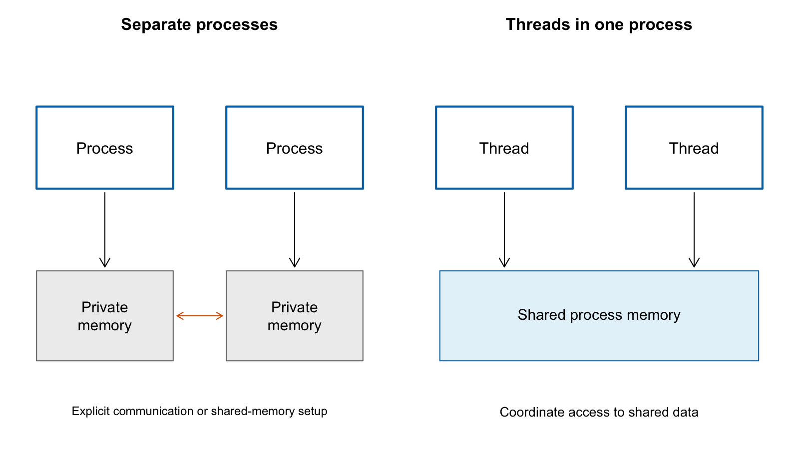
A thread (of execution) is a sequence of instructions to be run on a core.
Multiple threads can be part of the same process, and can thereby share resources with each other.
Distinct processes do not share resources (at least directly).
Processes and threads: memory
Types of parallelism
Running several processes in parallel (on one machine or several).
- May have machines connected via a network, with messages passed between them.
Running several threads in parallel within a process (on one machine).
Coarse parallel computing: lots of independent computations to do.
Just run them all in parallel in different processes. Speedup is simple.
If processes require lots of memory, may need to look at threads anyway.
Lightweight parallelism
Say you need to compute several numbers in a for loop, all of which are required for a subsequent step.
Then several threads can be used to each do some of the computations.
They share memory and are relatively lightweight to create/destroy in comparison to processes.
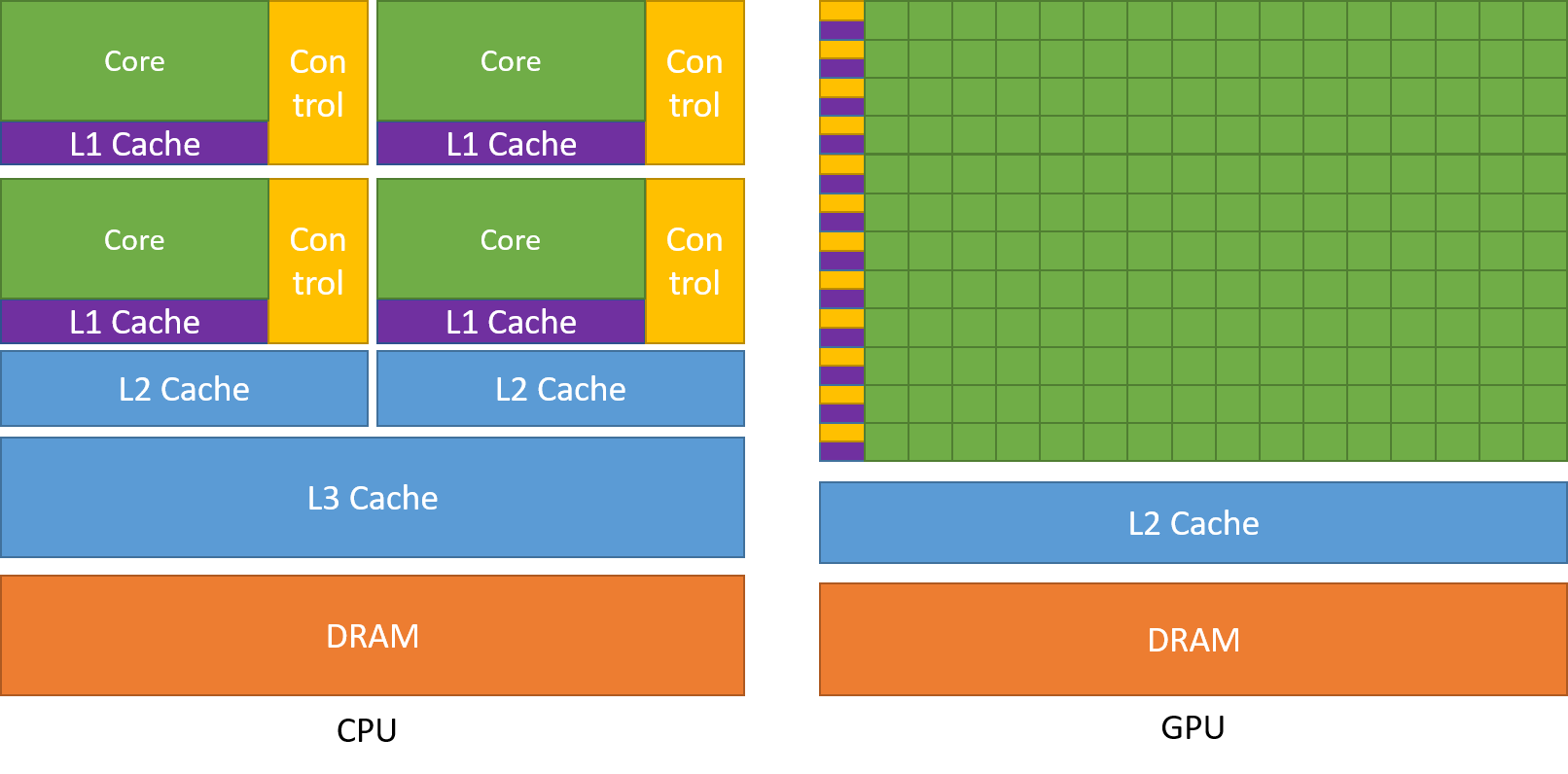
For GPUs, there are additional requirements for efficiency:
More ALUs/FPUs, less flow control.
Need blocks of computation to be identical, down to the instructions.
Also need memory to be laid out nicely for the computation.
In practice, people use frameworks to assist with / avoid GPU programming.
CPU vs GPU: transistor allocation
Memory management
High-level languages, e.g. R, Python.
Often we do “weird” things to enable fast computation, e.g. vectorizing computations in a way that necessitates the construction and destruction of arrays.
This is because we want to use “big” operations that have been compiled into machine code.
Instructions, from low-level languages like C and even Julia.
For loops are ideal.
Allocation of memory, e.g. for arrays is very slow.
This is important in serial computation, but more problematic in parallel.
Try optimizing code in Julia or C and see the difference!
An idea of memory costs
Rough speed of different types of memory access:
L1 cache (around 64KB) reference: 0.5ns.
L2 cache (around 256KB) reference: 7ns.
Main memory (around 48GB) reference: 100ns.
Disk seek: 10ms = \(10^{7}\)ns.
Solid State Drive: 0.1ms = \(10^{5}\) ns.
By analogy:
L1 cache: reaching for something on our desk (e.g. 1 second)
L2 cache: fetching it instead from a drawer (14 seconds)
Main memory: going up a set of stairs into another room to fetch something (3 minutes, 20 seconds).
Disk: walking from the University of Warwick to Cape Town (South Africa) and back (5555 hours or 231 days).
Solid state drive: walk to Brighton (55.55 hours or 2.31 days).
Limits to parallel speedup
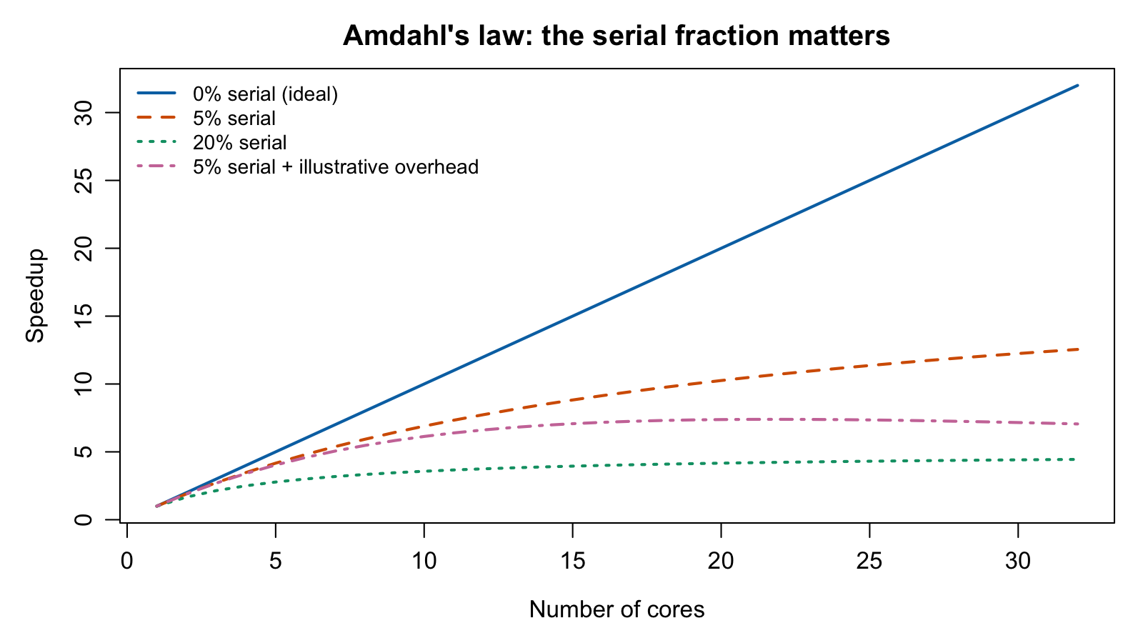
Serial work and communication can limit the benefit of more cores.
Complexity model
Simple model we often use to talk about algorithmic complexity:
- e.g. every operation (arithmetic, memory access, etc.) takes 1 unit of time.
Obviously not always accurate for certain types of computation.
For multi-threaded computation, some speedup is lost to overheads, synchronization, etc.
In some cases, different algorithms are appropriate for parallel computation.
Random algorithms
Random algorithms
A randomized algorithm uses an additional random input: its execution, output, or both may vary for a fixed problem input.
Randomized quicksort returns the same sorted values, but its comparisons and running time vary.
Monte Carlo integration returns a random approximation. Freivalds’ algorithm returns a random decision with a bounded error probability.
Here, "random algorithm" and "randomized algorithm" are synonyms.
Checking matrix multiplication
Say we have three \(n\times n\) matrices \(A\), \(B\) and \(C\).
We want to know if \(A\times B=C\).
Basic deterministic algorithm: compute \(A\times B\) in \(O(n^{3})\) time and check.
- Subcubic multiplication algorithms also exist; the randomized check avoids forming the product.
We will look at a way to check \(A\times B=C\) such that
If \(A\times B=C\), it always return “yes”.
If \(A\times B\neq C\), it returns “no” with probability at least \(\frac{1}{2}\), and “yes” otherwise.
Leads to \(\mathcal{O}(kn^{2})\) complexity with false positive error at most \(2^{-k}\).
Freivalds’ algorithm
If \(AB=C\), then \[ABx=A(Bx)=Cx.\]
So to check that \(AB=C\) we will generate a binary vector with independent Bernoulli(1/2) components, \(\xi\in\{0,1\}^{n}\).
Then we compute \(A(B\xi)\) and \(C\xi\) and return “yes” if all elements are equal and “no” otherwise.
This takes \(O(n^{2})\) time.
If \(AB=C\) then clearly we will always answer “yes”.
When \(AB\neq C\)
We check \(AB\xi=C\xi\) for \(\xi\sim{\rm Uniform}(\{0,1\}^{n})\).
This is like computing \(R=(AB-C)\xi\) and checking if \(R=0\).
If \(AB\neq C\) then \(D=(AB-C)\) has a non-zero element.
Let \(d_{ij}\) be a nonzero element of \(D\). We will look at \[\begin{eqnarray*} R_{i} & = & \sum_{k=1}^{n}d_{ik}\xi_{k}=d_{ij}\xi_{j}+\sum_{k=1,k\neq j}^{n}d_{ik}\xi_{k}=d_{ij}\xi_{j}+Y. \end{eqnarray*}\]
Now, \({\rm \mathbb{P}}\left(R_{i}=0\right)\) is equal to \[{\rm \mathbb{P}}\left(R_{i}=0|Y=0\right){\rm \mathbb{P}}\left(Y=0\right)+{\rm \mathbb{P}}\left(R_{i}=0|Y\neq0\right){\rm \mathbb{P}}\left(Y\neq0\right).\]
But \({\rm \mathbb{P}}\left(R_{i}=0|Y=0\right)={\rm \mathbb{P}}\left(\xi_{j}=0\right)=\frac{1}{2}\) and \({\rm \mathbb{P}}\left(R_{i}=0|Y\neq0\right)\leq{\rm \mathbb{P}}\left(\xi_{j}=1\right)=\frac{1}{2}\).
So \[{\rm Pr}\left(R_{i}=0\right)\leq\frac{1}{2}\left[{\rm Pr}\left(Y=0\right)+{\rm Pr}\left(Y\neq0\right)\right]=\frac{1}{2}.\]
When \(AB\neq C\)
When \(AB\neq C\), we will return “no” with probability at least \(\frac{1}{2}\).
Therefore, we can repeat the procedure with independent random vectors \(k\) times.
The probability that we do not observe a “no” but \(AB\neq C\) is at most \(2^{-k}\).
If we do observe a “no” we can output “no” and we are always right.
Freivalds: arithmetic assumptions
The probability guarantee assumes exact arithmetic, for example over a field.
With floating-point arithmetic, rounding can make an equality test reject a correct product.
A tolerance-based test needs a separate numerical error analysis.
Recap
Wrapping up
There are lots of topics we have not covered.
Unfortunately, many of these will be important to you!
Hopefully some coverage of fundamental ideas.
For research, we have to learn what is required to make progress.
Feedback welcome!