Numerical calculus I: Differentiation
It is not uncommon in statistical computing to need to compute derivatives of a function. For example, many optimization methods are gradient-based and so require computation of partial derivatives at various points in order to find local optima.
In these notes we will cover straightforward finite difference approaches as well as automatic differentiation.
1 Cancellation error
Consider the following R code
a <- 1e16
b <- 1e16 + pi
d <- b - a
so d should be \(\pi\), right? Actually
d[1] 4pi[1] 3.141593(d-pi)/pi[1] 0.2732395i.e. d is out by 27%.
This is an example of cancellation error. Almost any time we take the difference of two floating point numbers of similar magnitude (and sign) we find that the accuracy of the result is substantially reduced. The problem is rounding error. You can see what happens by considering computation to 16 places of decimals. Then \[
a = 1.0000000000000000 \times 10^{16} {\rm ~~~and~~~} b = 1.0000000000000003 \times 10^{16}
\] hence \(d=b-a=3\). (d was 4 above because the computer uses a binary rather than a decimal representation).
As we will see, derivative approximation is an area where we cannot ignore cancellation error as it is a pervasive issue. For example, cancellation error is the reason why \[ \sum_i x_i^2 - n \bar x^2 \] is not a good basis for a ‘one-pass’ method for calculating \[\sum_i (x_i-\bar x)^2.\] Indeed, \[\sum_i (x_i - x_1)^2 - n (\bar x - x_1)^2,\] is a simple one pass alternative, and generally much better. See, e.g., Chan et al. (1983).
Cancellation error is also a substantial issue in numerical linear algebra. For example, orthogonal matrix decompositions (used for QR, eigen and singular value decompositions), usually involve an apparently arbitrary choice at each successive rotation involved in the decomposition, about whether some element of the result of rotation should be positive or negative: one of the choices almost always involves substantially lower cancellation error than the other, and is the one taken.
Since approximation of derivatives inevitably involves subtracting similar numbers, it is self evident that cancellation error will cause some difficulty. Numerical integration tends to be a more stable process (at least when integrating positive functions) because numerical integration is basically about adding numbers up, rather than looking at differences between them, and this is more stable. Consider, e.g.
f <- a + b
(f-2e16-pi)/(2e16+pi) ## relative error in sum, is tiny...
[1] 4.292037e-172 Gradients, partial derivatives and derivatives
Recall that the derivative of a function \(f : \mathbb{R} \to \mathbb{R}\) is the function \(f'\) given by \[ f'(x) = \lim_{h\to 0} \frac{f(x+h)-f(x)}{h}, \tag{1}\] if the limit exists.
The gradient of some function \(f : \mathbb{R}^d \to \mathbb{R}\) is the vector of partial derivatives \[ \left ( \frac{\partial f}{\partial x_1}, \ldots, \frac{\partial f}{\partial x_d} \right ), \] where \[ \frac{\partial f}{\partial x_i}({\bf a}) = \lim_{h\to 0} \frac{f(a_1,\ldots,a_{i-1},a_i+h,a_{i+1},\ldots,a_d)-f({\bf a})}{h}. \] In other words, \(\partial f / \partial x_i\) is the derivative of the function with respect to the \(i\)th variable with the others held constant.
Hence, approximating a gradient can be done by approximating each partial derivative. In particular, for the sake of clarity we can often reduce our attention to \(f : \mathbb{R} \to \mathbb{R}\).
Although we will focus on this simple setting, it is nevertheless worth remembering that in practice one could be approximating gradients of very complicated functions with large \(d\), e.g. the log-likelihood associated with a very complex statistical model with lots of parameters.
3 Approximate derivatives by finite differencing
A natural approximation of Equation 1 is \[ f'_h(x) = \frac{f(x+h)-f(x)}{h}, \] with \(h\) “suitably small”.
Taylor’s Theorem gives \[ f(x+h) = f(x) + hf'(x) + \frac{1}{2} h^2 f''(\xi), \] where \(\xi \in (x,x+h)\). Rearranging, and assuming \(\sup_z|f''(z)| \leq L\), we have \[ \left | \frac{f(x+h)-f(x)}{h} - f'(x) \right | = \frac{1}{2}h | f''(\xi) | \leq \frac{Lh}{2}. \tag{2}\] This gives us a bound on the error obtained by using some fixed \(h > 0\) rather than taking the limit.
Of course, in reality we cannot compute \(f\) pointwise exactly. Suppose that we actually compute \(\tilde{f}\) instead of \(f\), and it has a relative error of \(\epsilon\), i.e. for all \(x\), \[ |\tilde{f}(x)-f(x)| \leq \epsilon |f(x)|. \] In practice \(\epsilon\) could be something like machine precision, but of course it depends on how \(\tilde{f}\) is related to \(f\).
Then if \(\sup_z |f(z)| \leq L_f\), we obtain \[ \left | \frac{\tilde{f}(x+h)-\tilde{f}(x)}{h} - \frac{f(x+h)-f(x)}{h} \right | \leq 2\frac{\epsilon L_f}{h}, \tag{3}\] giving a bound for the cancellation error. This is bounding the difference between what we actually compute and the idealized \(f'_h\).
An application of the triangle inequality allows us to combine Equation 2 and Equation 3 to obtain \[ \left | \frac{\tilde{f}(x+h)-\tilde{f}(x)}{h} - f'(x) \right | \leq \frac{L h}{2} + \frac{2 \epsilon L_f }{h}. \] Minimizing the bound involves trading off the two sources of error, and a simple analysis gives \[ h = \sqrt{\frac{4\epsilon L_f}{L}}, \] suggesting that if the typical size of \(f\) and its second derivatives are similar then \(h \approx \epsilon^{1/2}\) is the right kind of scaling. This is why the square root of the machine precision is often used as the finite difference interval.
As always,note the assumptions: we require that \(L_f \approx L\) and \(f\) to be calculable to a relative accuracy that is a small multiple of the machine precision for such a choice to work well. More generally, the analysis above suggests choosing a particular \(h\) for different \(x\) when trying to approximate \(f'(x)\). This may or may not be practical. For more information, see Gill, Murray and Wright (1981).
3.1 Other FD formulae
The finite difference approach considered above is forward differencing. Centred differences are more accurate, but can be more costly depending on the context \[ f'_h(x) = \frac{f(x+h)-f(x-h)}{2h}, \] in the setting analyzed above \(h \approx \epsilon^{1/3}\) is about right.
Sometimes it is useful to approximate higher order derivatives. For example \[ f''_h(x) = \frac{f(x+h)-2f(x) + f(x-h)}{h^2}, \] can be used as an approximation for \(f''(x)\) and the analysis above can be extended to suggest \(h \approx \epsilon^{1/4}\).
4 Automatic Differentiation: code that differentiates itself
Differentiation of complex models or other expressions is tedious, but ultimately routine. One simply applies the chain rule and some known derivatives, repeatedly. At its essence is the fact that even complicated computations can be reduced to a sequence of elementary arithmetic operations and function evaluations. The main problem with doing this is the human speed, error rate and limits on human patience. Given that differentiation is just the repeated application of the chain rule and known derivatives, couldn’t it be automated? The answer is yes.
There are two approaches. The first is symbolic differentiation using a computer algebra package such as Maple or Mathematica. This works, but can produce enormously unwieldy expressions when applied to a complex function. The problem is that the number of terms in a symbolic derivative can be very much larger than for the expression being evaluated. It is also very difficult to apply to a complex simulation model, for example.
The second approach is automatic differentiation. This operates by differentiating a function based directly on the computer code that evaluates the function. There are several different approaches to this, but many use the features of object oriented programming languages to achieve the desired end. The key feature of an object oriented language, from the AD perspective, is that every data structure, or object in such a language has a class and the meaning of operators such as +, -, *, etc. depends on the class of the objects to which they are applied. Similarly the action of a function depends on the class of its arguments.
Suppose then, that we would like to differentiate \[ f(x_1,x_2,x_3) = \left (x_1 x_2 \sin(x_3) + e^{x_1x_2} \right )/x_3 \] w.r.t. its real arguments \(x_1\), \(x_2\) and \(x_3\). This example is taken from Nocedal and Wright, (2006). In R the code
(x1*x2*sin(x3) + exp(x1*x2))/x3would evaluate the function, if x1, x2 and x3 were initialised to be floating point numbers.
We can define a new type of object of class ad which has a value (a floating point number) and a grad attribute. In the current case this grad attribute will be a 3-vector containing the derivatives of the value w.r.t. x1, x2 and x3. We can now define versions of the arithmetic operators and mathematical functions which will return class ad results with the correct value and grad attribute, whenever they are used in an expression.
Here is an R function to create and initialise a simple class ad object
ad <- function(x,diff = c(1,1)) {
## create class "ad" object. diff[1] is length of grad
## diff[2] is the element of grad to initialize to 1, the rest to 0.
  grad <- rep(0,diff[1])
  if (diff[2]>0 && diff[2]<=diff[1]) grad[diff[2]] <- 1
  attr(x,"grad") <- grad
  class(x) <- "ad"
  x
}
Here it is in use, initialising x1 to the value 1, giving it a 3 dimensional grad attribute, and setting the first element of grad to 1 since \(\partial x_1 / \partial x_1 =1\).
x1 <- ad(1,c(3,1))
x1
[1] 1
attr(,"grad")
[1] 1 0 0
attr(,"class")
[1] "ad"Now the interesting part. We can define versions of mathematical functions and operators that are specific to class ad objects and correctly propagate derivatives alongside values. Here is a \(\sin\) function for class ad.
sin.ad <- function(a) {
  grad.a <- attr(a,"grad")
  a <- as.numeric(a) ## avoid infinite recursion - change class
  d <- sin(a)
  attr(d,"grad") <- cos(a) * grad.a ## chain rule
  class(d) <- "ad"
  d
}
and here is what happens when it is applied to x1
sin(x1)[1] 0.841471
attr(,"grad")
[1] 0.5403023 0.0000000 0.0000000
attr(,"class")
[1] "ad"i.e. the value of the result is \(\sin(x_1)\), while the first element of its grad attribute contains the derivative of \(\sin(x_1)\) w.r.t. \(x_1\) evaluated at \(x_1=1\).
Operators can also be overloaded in this way. e.g. here is multiplication operator for class ad:
"*.ad" <- function(a,b) { ## ad multiplication
  grad.a <- attr(a,"grad")
  grad.b <- attr(b,"grad")
  a <- as.numeric(a)
  b <- as.numeric(b)
  d <- a*b    ## evaluation
  attr(d,"grad") <- a * grad.b + b * grad.a ## product rule
  class(d) <- "ad"
  d
}
Continuing in the same way we can provide a complete library of mathematical functions and operators for the ad} class. Given such a library, we can obtain the derivatives of a function directly from the code that would simply evaluate it, given ordinary floating point arguments. For example, here is some code evaluating a function.
  x1 <- 1; x2 <- 2; x3 <- pi/2
  (x1*x2*sin(x3)+ exp(x1*x2))/x3
[1] 5.977259and here is the same code with the arguments replaced by ad objects
  x1 <- ad(1, c(3,1))
  x2 <- ad(2, c(3,2))
  x3 <- ad(pi/2, c(3,3))
  (x1*x2*sin(x3) + exp(x1*x2))/x3
[1] 5.977259
attr(,"grad")
[1] 10.681278 5.340639 -3.805241
attr(,"class")
[1] "ad"you can check that these results are correct (to machine accuracy).
This simple propagation of derivatives alongside the evaluation of a function is known as forward mode auto-differentiation. R is not the best language in which to try to do this, and if you need AD it is much better to use existing software libraries in C++, for example, which have done all the function and operator re-writing for you.
4.1 Reverse mode AD
If you require many derivatives of a scalar valued function then forward mode AD will have a theoretical computational cost similar to finite differencing, since at least as many operations are required for each derivative as are required for function evaluation. In reality the overheads associated with operator overloading make AD more expensive (alternative strategies also carry overheads). Of course the benefit of AD is higher accuracy, and in many applications the cost is not critical.
An alternative with the potential for big computational savings over finite differencing is reverse mode AD. To understand this it helps to think of the evaluation of a function in terms of a computational graph. Again concentrate on the example function given in Nocedal and Wright (2006): \[ f(x_1,x_2,x_3) = \left (x_1 x_2 \sin(x_3) + e^{x_1x_2} \right )/x_3 \] Any computer evaluating this must break the computation down into a sequence of elementary operations on one or two floating point numbers. This can be thought of as a graph:
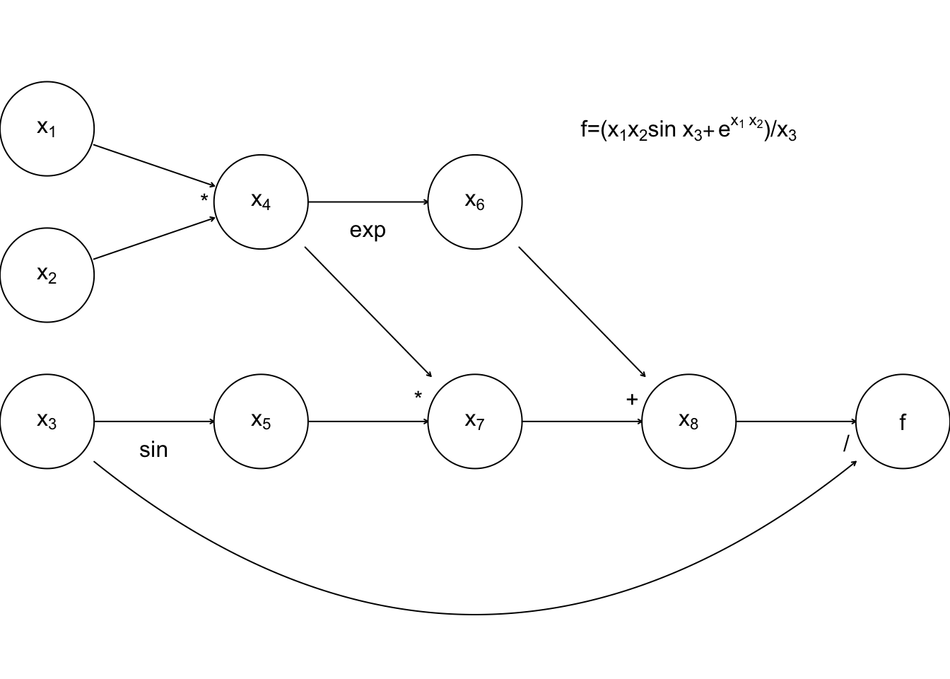
where the nodes \(x_4\) to \(x_8\) are the intermediate quantities that will have to be produced en route from the input values \(x_1\) to \(x_3\) to the final answer, \(f\). The arrows run from parent nodes to child nodes. No child can be evaluated until all its parents have been evaluated.
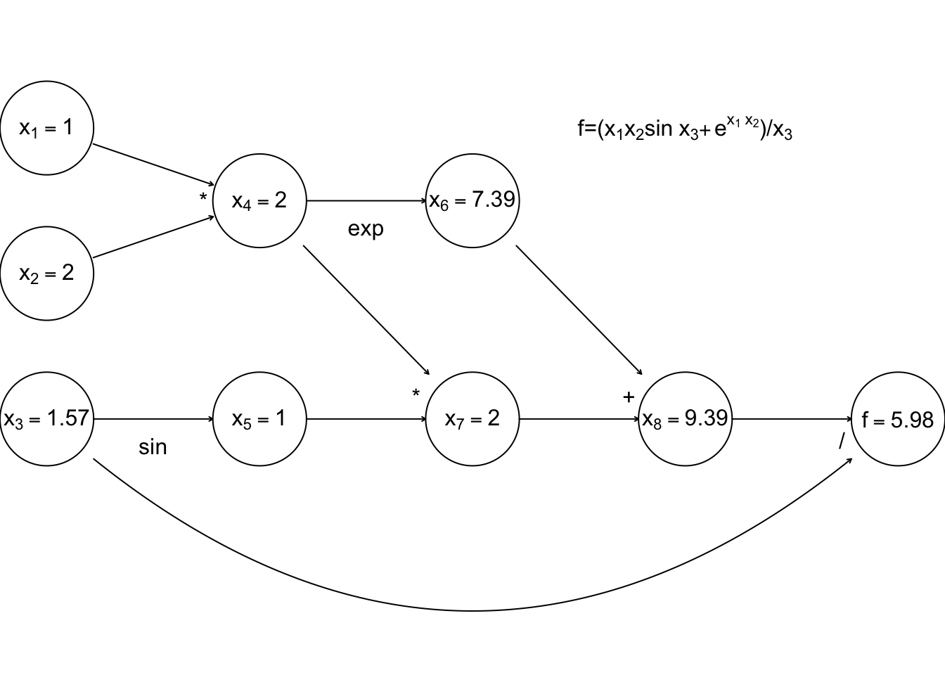
Simple left to right evaluation of this graph results in this
Now, forward mode AD carries derivatives forward through the graph, alongside values. e.g. the derivative of a node with respect to input variable, \(x_1\) is computed using \[ \frac{\partial x_k}{\partial x_1} = \sum_{j~{\rm parent~of~}k} \frac{\partial x_k}{\partial x_j}\frac{\partial x_j}{\partial x_1} \] (the r.h.s. being evaluated by overloaded functions and operators, in the object oriented approach). The following illustrates this process, just for the derivative w.r.t. \(x_1\).
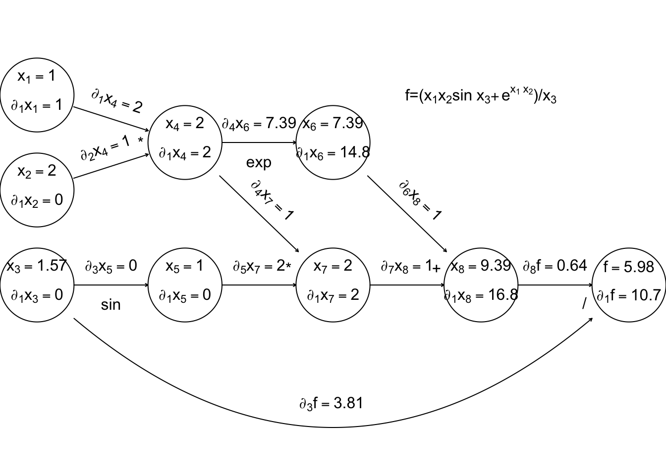
Again computation runs left to right, with evaluation of a node only possible once all parent values are known.
Now, if we require derivatives w.r.t. several input variables, then each node will have to evaluate derivatives w.r.t. each of these variables, and this becomes expensive (in terms of the previous graph, each node would contain multiple evaluated derivatives). Reverse mode therefore does something ingenious. It first executes a forward sweep through the graph, evaluating the function and all the derivatives of nodes w.r.t. their parents.
The reverse sweep then works backwards through the graph, evaluating the derivative of \(f\) w.r.t. each node, using the following \[ \frac{\partial f}{\partial x_k} = \sum_{j{\rm~is~child~of~k}} \frac{\partial x_j}{\partial x_k} \frac{\partial f}{\partial x_j} \] and the fact that at the terminal node \(\partial f/{\partial f } = 1\).
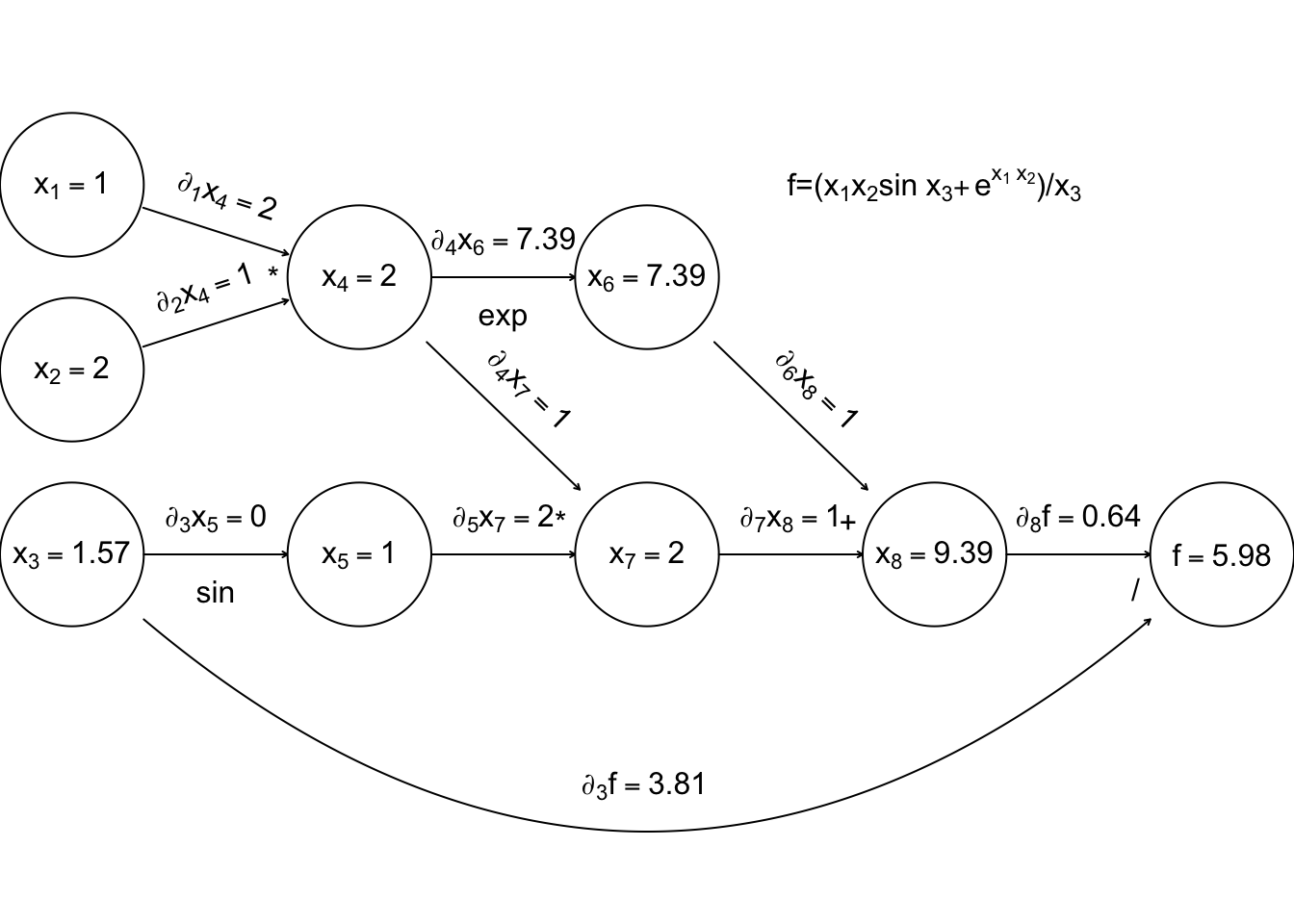
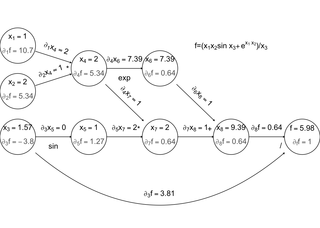
The derivatives in grey are those calculated on the reverse sweep. The point here is that there is only one derivative to be evaluated at each node, but in the end we know the derivative of \(f\) w.r.t. every input variable. Reverse mode can therefore save a large number of operations relative to finite differencing or forward mode. Once again, general purpose AD libraries automate the process for you, so that all you need to be able to write is the evaluation code.
Unfortunately reverse mode efficiency comes at a heavy price. In forward mode we could discard the values and derivatives associated with a node as soon as all its children were evaluated. In reverse mode the values of all nodes and the evaluated derivatives associated with every connection have to be stored during the forward sweep, in order to be used in the reverse sweep. This is a heavy storage requirement. For example, if \(f\) involved the inversion of a \(1000\times1000\) matrix then we would have to store some \(2 \times 10^9\) intermediate node values plus a similar number of evaluated derivatives. That is some 32 Gigabytes of storage before we even consider the requirements for storing the structure of the graph.
4.2 A caveat
For AD to work it is not sufficient that the function being evaluated has properly defined derivatives at the evaluated function value. We require that every function/operator used in the evaluation has properly defined derivatives at its evaluated argument(s). This can create a problem with code that executes conditional on the value of some variable. For example the Box-Cox transformation of a positive datum \(y\) is \[ B(y;\lambda) = \left \{ \begin{array}{ll} (y^\lambda - 1)/\lambda & \lambda \ne 0\\ \log(y) & \lambda = 0 \end{array} \right . \] This is a continuously differentiable function of \(\lambda\) for all \(\lambda \in \mathbb {R}\). However, if you code this up in the obvious way then AD will never get the derivative of \(B\) w.r.t. \(\lambda\) right if \(\lambda = 0\). To be precise, one can see that \[ \frac{\partial}{\partial \lambda} B(y;0) = \lim_{h \to 0} \frac{(y^h-1)/h - \log(y)}{h} = \frac{\log(y)^2}{2}, \] but this cannot be recovered in the manner described above by evaluating \(B(y;0)\).
4.3 Using AD to improve FD
When fitting complicated or computer intensive models it can be that AD is too expensive to use for routine derivative calculation during optimization. However, with the gradual emergence of highly optimized libraries, this situation is changing, and in any case it can still provide a useful means for calibrating FD intervals. A ‘typical’ model run can be auto-differentiated, and the finite difference intervals adjusted to achieve the closest match to the AD derivatives. As optimization progresses one or two further calibrations of the FD intervals can be carried out as necessary.
5 Further reading on computer integration and differentiation
Chapter 8 of Nocedal, J. & S.J. Wright (2006) Numerical Optimization (2nd ed.), Springer, offers a good introduction to finite differencing and AD, and the AD examples above are adapted directly from this source.
Gill, P.E. , W. Murray and M.H. Wright (1981) Practical Optimization Academic Press, Section 8.6 offers the treatment of finite differencing that you should read before using it on anything but the most benign problems. This is one of the few references that tells you what to do if your objective is not `well scaled’.
Griewank, A. (2000) Evaluating Derivatives: Principles and Techniques of Algorithmic Differentiation SIAM, is the reference for Automatic Differentiation. If you want to know exactly how AD code works then this is the place to start. It is very clearly written and should be consulted before using AD on anything seriously computer intensive.
http://www.autodiff.org is a great resource for information on AD and AD tools.
If you want to see AD in serious action, take a look at e.g. Kalnay, E (2003) Atmospheric Modelling, Data Assimilation and Predictability.
R is not the best language for computational statistics, and automatic differentiation is not particularly well supported. There are better automatic differentiation options in Julia and Python. The JAX library for Python is particularly interesting https://jax.readthedocs.io/
Although most widely-used AD libraries are based on object-oriented programming approaches, arguably the most elegant approaches exploit functional programming languages with strong static type systems. See, for example: Elliott, C. (2018) The simple essence of automatic differentiation. Proc. ACM Program. Lang. 2, ICFP, Article 70., and the Dex language.
Chapter 10 of Monahan, J.F (2001) Numerical Methods of Statistics, offers more information on numerical integration, including much of the detail skipped over here, although it is not always easy to follow, if you don’t already have quite a good idea what is going on.
Lange, K (2010) Numerical Analysis for Statisticians, 2nd ed., Springer. Chapter 18 is good on one-dimensional quadrature.
Ripley, B.D. (1987, 2006) Stochastic Simulation Chapters 5 and section 7.4 are good discussions of stochastic integration and Quasi Monte Carlo integration.
Robert, C.P. and G. Casella (1999) Monte Carlo Statistical Methods Chapter 3 (and beyond) goes into much more depth than these notes on stochastic integration.
Press et al. (2007) Numerical Recipes (3rd ed), Cambridge, has a nice chapter on numerical integration, but with emphasis on 1D.