Introduction

In combination, modern computer hardware, algorithms and numerical methods are extraordinarily impressive. Take a moment to consider some simple examples, all using R.

Simulate a million random numbers and then sort them into ascending order.
```
x <- runif(1000000)
system.time(xs <- sort(x))
```
```
   user  system elapsed 
  0.131   0.014   0.151 
```
The sorting operation takes a fraction of a second on a laptop. If each of the numbers in x had been written on its own playing card, the resulting stack of cards would have been 40 metres high. Imagine trying to sort x without computers and clever algorithms.
Here is a matrix calculation of comparatively modest dimension, by modern statistical standards.
```
set.seed(2)
n <- 1000
A <- matrix(runif(n*n),n,n)
system.time(Ai <- solve(A))  # invert A
```
```
   user  system elapsed 
  2.029   0.067   2.275 
```
```
range(Ai%*%A-diag(n))        # check accuracy of result
```
```
[1] -1.462719e-12  1.457834e-12
```
The matrix inversion took under half a second to perform, and the inverse satisfied its defining equations to around one part in $10^{11}$. It involved around 2 billion ($2 \times 10^9$) basic arithmetic calculations (additions, subtractions multiplications or divisions). At a very optimistic 10 seconds per calculation this would take 86 average working lives to perform without a computer (and that’s assuming we use the same algorithm as the computer, rather than Cramer’s rule, and made no mistakes). Checking the result by multiplying the A by the resulting inverse would take another 86 working lives.

The preceding two examples are problems in which smaller versions of the same problem can be solved more or less exactly without computers and special algorithms or numerical methods. In these cases, computers allow much more useful sizes of problem to be solved very quickly. Not all problems are like this, and some problems can really only be solved by computer. For example, here is a scaled version of a simple delay differential equation model of adult population size, $n$, in a laboratory blowfly culture. \[ \frac{{\rm d}n}{{\rm d}t} = PT_D n(t-1) e^{-n(t-1)} - \delta T_D n(t). \] The dynamic behaviour of the solutions to this model is governed by parameter groups $PT_D$ and $\delta T_D$, but the equation cannot be solved analytically, from any interesting set of initial conditions. To see what solutions actually look like we must use numerical methods.

#install.packages("PBSddesolve") ## install package from CRAN

library(PBSddesolve)


-----------------------------------------------------------
PBSddesolve 1.13.4 -- Copyright (C) 2007-2024 Fisheries and Oceans Canada
(based on solv95 by Simon Wood)

A complete user guide 'PBSddesolve-UG.pdf' is located at 
/Users/al17824/Library/R/x86_64/4.4/library/PBSddesolve/doc/PBSddesolve-UG.pdf

Demos include 'blowflies', 'cooling', 'icecream', and 'lorenz'
They can be run two ways:

1. Using 'utils' package 'demo' function, run command
> demo(icecream, package='PBSddesolve', ask=FALSE)

2. Using package 'PBSmodelling', run commands
> require(PBSmodelling); runDemos()
and choose PBSddesolve and then one of the four demos.

Packaged on 2024-01-04
Pacific Biological Station, Nanaimo

All available PBS packages can be found at
https://github.com/pbs-software
-----------------------------------------------------------

bfly <- function(t,y,parms) {
## function defining rate of change of blowfly population, y, at
## time t, given y, t, lagged values of y form `pastvalue' and
## the parameters in `parms'. See `ddesolve' docs for more details.

## making names more useful ...
  P <- parms$P;d <- parms$delta;y0 <- parms$yinit

  if (t<=1) y1 <- P*y0*exp(-y0)-d*y else { ## initial phase
    ylag <- pastvalue(t-1)         ## getting lagged y
    y1 <- P*ylag*exp(-ylag) - d*y  ## the gradient
  }
  y1  ## return gradient
}

## set parameters...
parms <- list(P=150,delta=6,yinit=2.001)
## solve model...
yout <- dde(y=parms$yinit,times=seq(0,15,0.05),func=bfly,parms=parms)
## plot result...
plot(yout$time,yout$y1,type="l",ylab="n",xlab="time")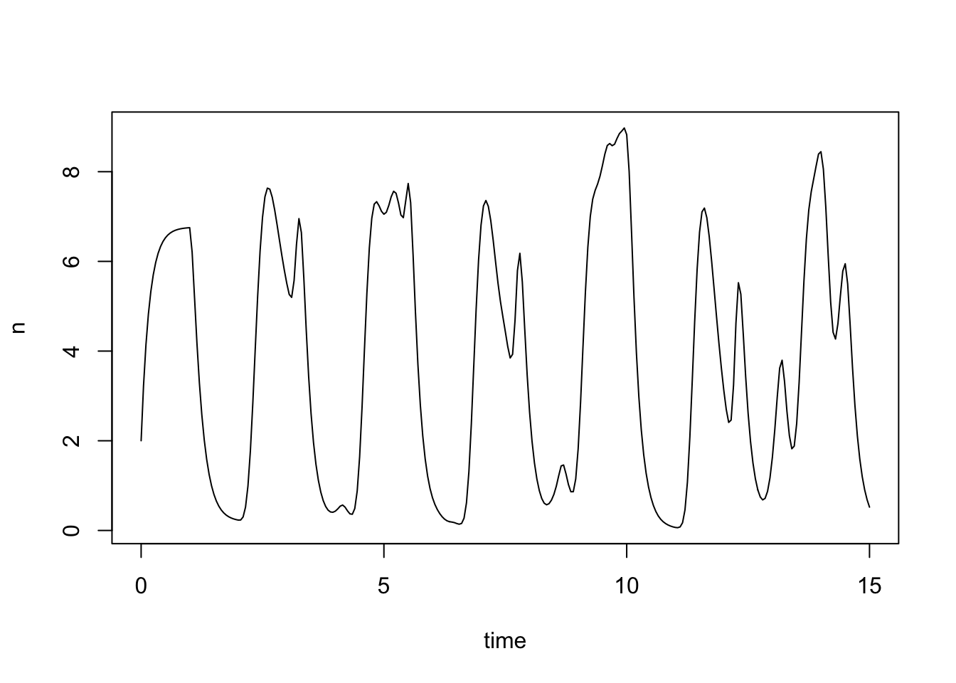

Here the solution of the model (to an accuracy of 1 part in $10^8$), took a quarter of a second.

1 Things can go wrong

The amazing combination of speed and accuracy apparent in many computer algorithms and numerical methods can lead to a false sense of security and the wrong impression that in translating mathematical and statistical ideas into computer code we can simply treat the numerical methods and algorithms we use as infallible `black boxes’. This is not the case, as the following three simple examples should illustrate. You may be able to figure out the cause of the problem in each case, but don’t worry if not: we will return to each of the examples in the course.

The system.time function in R measures how long a particular operation takes to execute. First generate two $2000 \times 2000$ matrices, $\bf A$ and $\bf B$ and a vector, $\bf y$.

n <- 2000
A <- matrix(runif(n*n),n,n)
B <- matrix(runif(n*n),n,n)
y <- runif(n)

Now form the product $\bf ABy$ in two slightly different ways

system.time(f0 <- A%*%B%*%y)

   user  system elapsed 
 10.094   0.260  10.895

system.time(f1 <- A%*%(B%*%y))

   user  system elapsed 
  0.015   0.000   0.017

f0 and f1 are identical, to machine precision, so why is one calculation so much quicker than the other? Clearly anyone wanting to compute with matrices had better know the answer to this.

Note that benchmarking using one replicate is a bit crude. There are various R packages that can facilitate benchmarking and profiling of R code. Here we illustrate use of the rbenchmark package, which is available on CRAN.

library(rbenchmark)
benchmark(
    "ABy" = {
        f0 <- A%*%B%*%y
    },
    "A(By)" = {
        f1 <- A%*%(B%*%y)
    },
    replications = 10,
    columns = c("test", "replications", "elapsed",
                "relative", "user.self", "sys.self"))

   test replications elapsed relative user.self sys.self
2 A(By)           10   0.256    1.000     0.197    0.009
1   ABy           10 121.996  476.547   105.282    3.255

It is not unusual to require derivatives of complicated functions, for example when estimating models. Such derivatives can be very tedious or difficult to calculate directly, but can be approximated quite easily by `finite differencing’. e.g. if $f$ is a function of $x$ then \[ \frac{\partial{f}}{\partial{x}} \simeq \frac{f(x+\Delta) - f(x)}{\Delta} \] where $\Delta$ is a small interval. Taylor’s theorem implies that the right hand side tends to the left hand side, above, as $\Delta \to 0$. It is easy to try this out on an example where the answer is known, so consider differentiating $\sin(x)$ w.r.t. $x$.
```
x <- seq(1,2*pi,length=1000)
delta <- 1e-3  ## FD interval
dsin.dx <- (sin(x+delta)-sin(x))/delta ## FD derivative
error <- dsin.dx-cos(x)  ## error in FD derivative
```
The following plots the results. On the LHS $\sin(x)$ is dashed, it’s true derivative $\cos(x)$ is dotted and the FD derivative is continuous. The RHS shows the difference between the FD approximation and the truth.

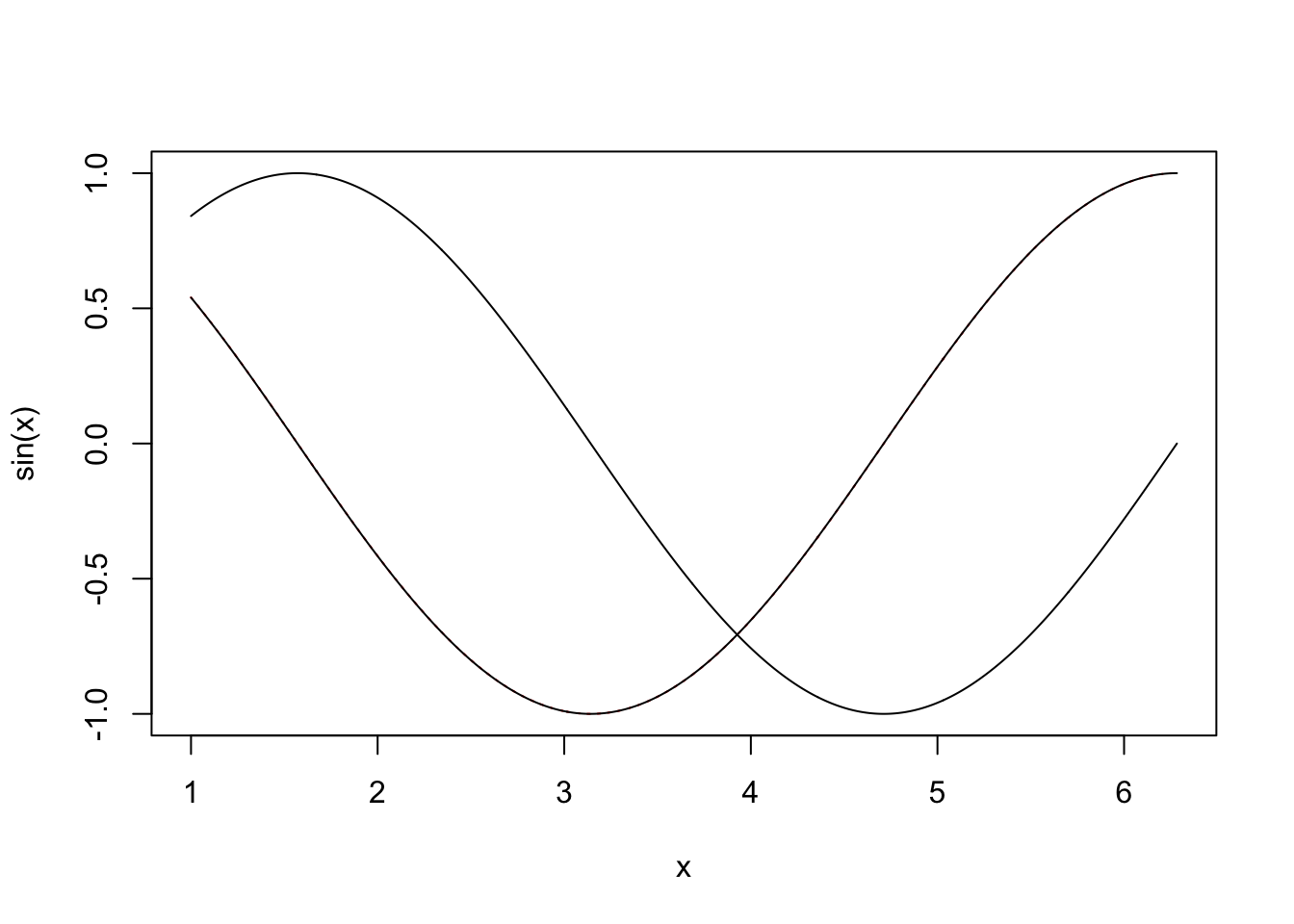
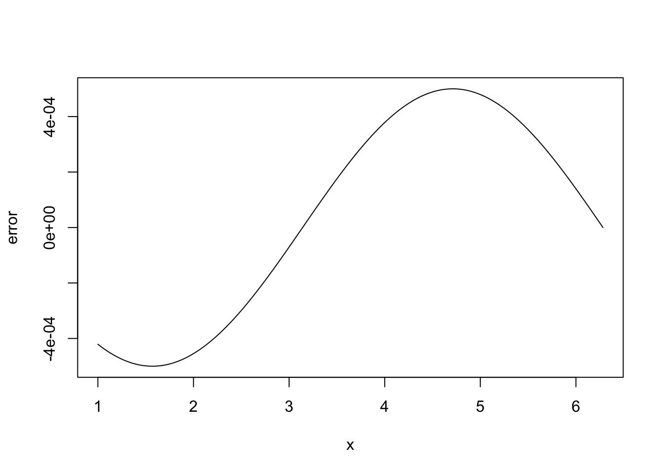
Note that the error appears to be of about the same magnitude as the finite difference interval $\Delta$. Perhaps we could reduce the error to around the machine precision by using a much smaller $\Delta$. Here is the equivalent of the previous plot, when delta is 1e-15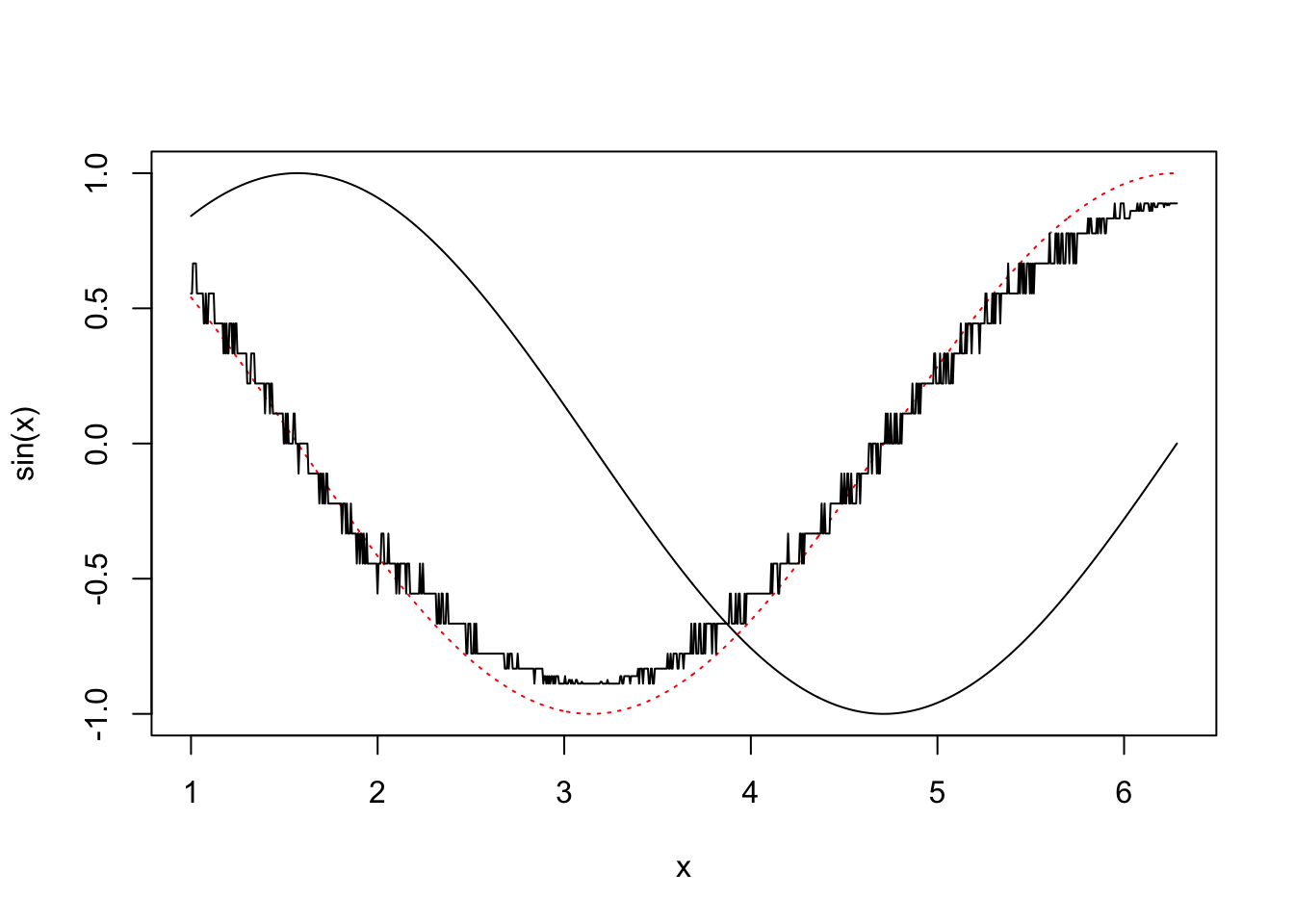

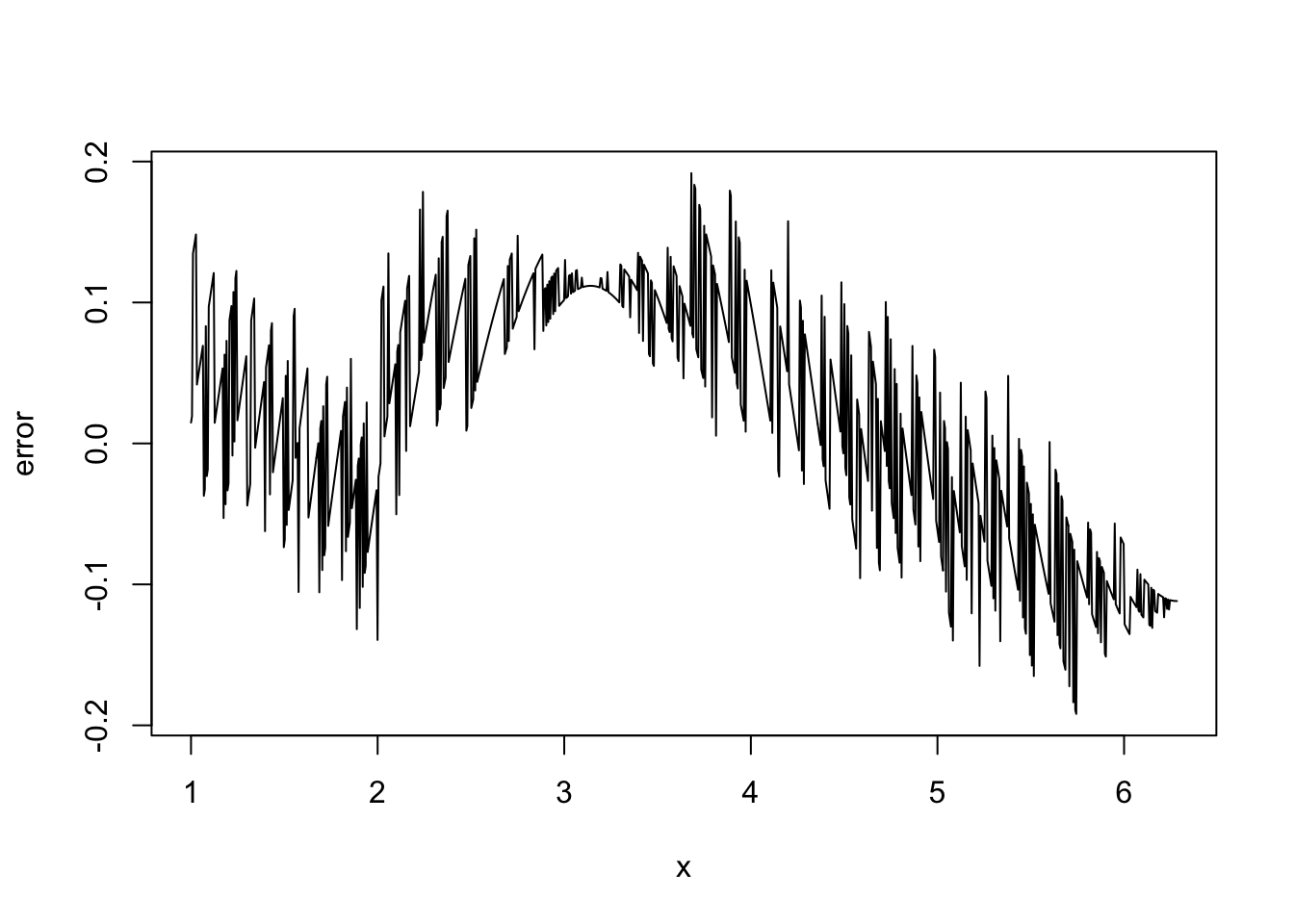
Clearly there is something wrong with the idea that decreasing $\Delta$ must always increase accuracy here.
Consider the data generated by this code:
```
set.seed(1); n <- 100
xx <- sort(runif(n))
y <- .2*(xx-.5)+(xx-.5)^2 + rnorm(n)*.1
x <- xx+100
plot(x,y)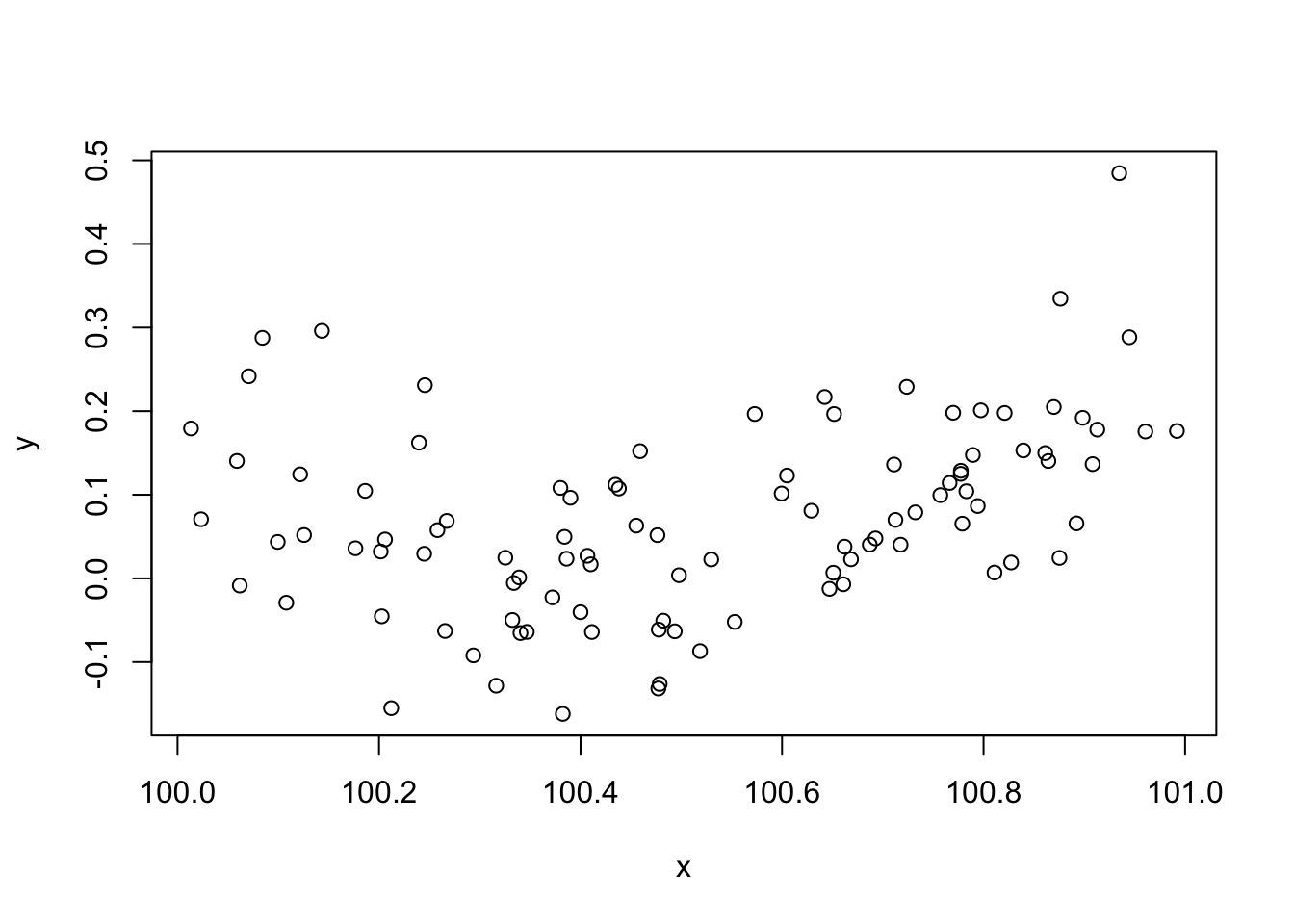
```
An appropriate and innocuous linear model for these data is $y_i = \beta_0 + \beta_1 x_i + \beta_2 x_i^2 + \epsilon_i$, where the $\epsilon_i$ are independent, zero mean constant variance r.v.s and the $\beta_j$ are parameters. This can be fitted in R, and the curve plotted, with
```
b <- lm(y~x+I(x^2))
plot(x,y)
lines(x,b$fitted.values,col="red")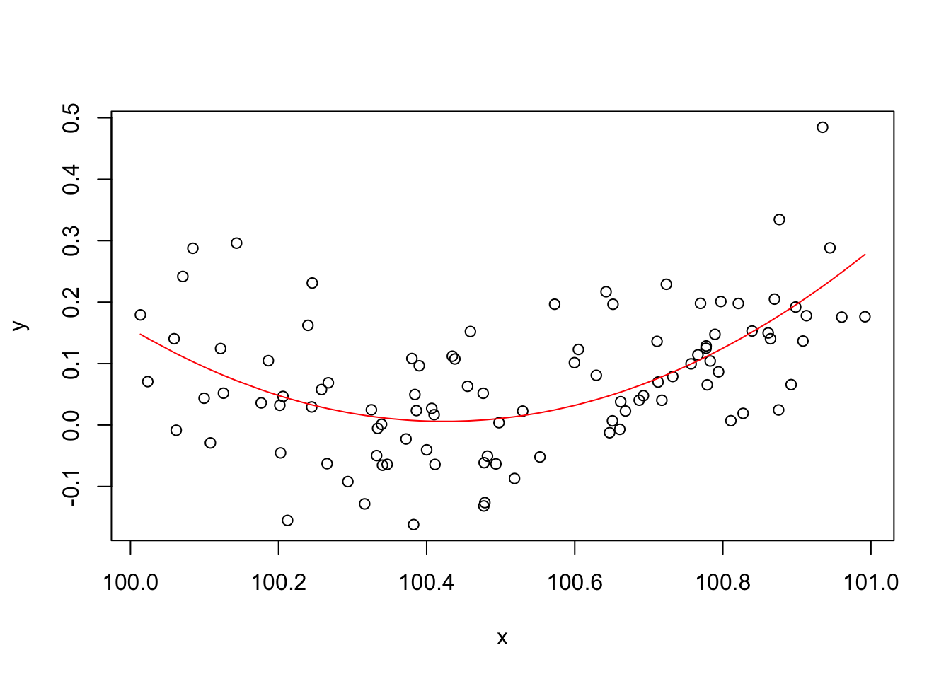
```
From basic statistical modelling courses, recall that the least squares parameter estimates for a linear model are given by $\hat {\boldsymbol{\beta}}= ({\bf X}^{\sf T}{\bf X})^{-1}{\bf X}^{\sf T}{\bf y}$ where ${\bf X}$ is the model matrix. An alternative to use of lm would be to use this expression for $\hat {\boldsymbol{\beta}}$ directly.
```
X <- model.matrix(b) ## get same model matrix used above
## direct solution of `normal equations'
beta.hat <- solve(t(X)%*%X,t(X)%*%y) 
```
```
Error in solve.default(t(X) %*% X, t(X) %*% y): system is computationally singular: reciprocal condition number = 3.9864e-19
```
Something has gone badly wrong here, and this is a rather straightforward model. It’s important to understand what has happened before trying to write code to apply more sophisticated approaches to more complicated models.

In case you are wondering, one can make lm fail too. Mathematically it is easy to show that the model fitted values should be unchanged if I simply add 900 to the x values, but if I refit the model to such shifted data using lm then the following fitted values result, which can not be correct.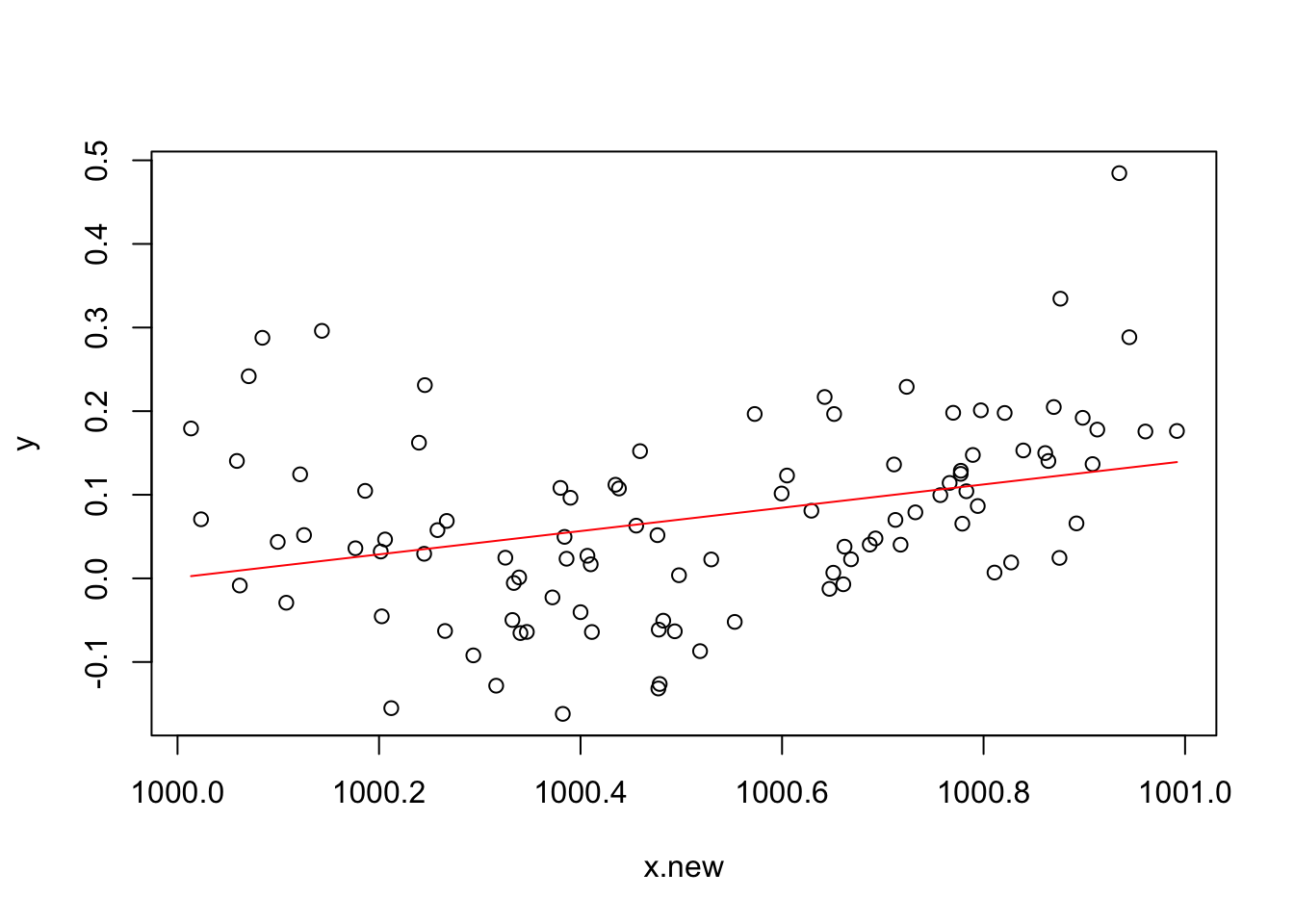

In particular, in this case lm estimates the coefficient of $x^2$ as NA due to numerical issues.