Numerical Calculus II: Integration
December 2025
Outline
- Introduction
- Quadrature
- Deterministic approximation
- Monte Carlo
- Recap
Introduction
Introduction
Integration is involved in, for example:
integrating random effects out of a joint distribution to get a likelihood,
evaluating expectations, including posterior expectations in Bayesian inference.
Unfortunately, integration is typically intractable and accurate approximations are often computationally expensive.
There is no simple rule for obtaining the integral of a composition of functions, cf. differentiation and the chain rule.
We will look at two approaches:
one more classical, for integrating 1D functions and,
one based on viewing integrals as expectations of random variables.
Quadrature
Integrals
The definite integral of a function \(f\) over the interval \((a,b)\) is \[I(f)=\int_{a}^{b}f(x){\rm d}x.\]
Our goal in quadrature is to approximate this integral with a sum \[\sum_{i=1}^{N}w_{i}f(x_{i}),\] for some choice of \(\{(x_{i},w_{i}):i\in\{1,\ldots,N\}\}\).
How can we come up with some suitable points and weights?
Polynomial approximations
Approximate \(f\) by a polynomial \(p\): its integral \(I(p)\) can be computed exactly.
For distinct nodes \(x_{1},\ldots,x_{k}\), the unique interpolating polynomial has degree at most \(k-1\):
\[p_{k-1}(x)=\sum_{i=1}^{k}\ell_{i}(x)f(x_{i}),\qquad\ell_{i}(x)=\prod_{j\ne i}\frac{x-x_{j}}{x_{i}-x_{j}}.\]
- Integrating the basis polynomials gives weights for a quadrature rule.
Example interpolating polynomials
Piecewise interpolating polynomials
For finite \(k\), the error \(\left\Vert f-p_{k-1}\right\Vert\) may be large.
Options: increase \(k\) or split the domain into subintervals.
- Piecewise polynomial approximation.
Simple version: split into \(m\) subintervals and use \(k\) equally spaced points in each subinterval.
- Closed if we put points at the interval boundaries. Open if we don’t.
Course website again.
Integrating the polynomials
Consider integrating an interpolating polynomial \(p_{k-1}\): \[\begin{align*} I(p_{k-1}) & =\int_{a}^{b}p_{k-1}(x){\rm d}x\\ & =\int_{a}^{b}\sum_{i=1}^{k}\ell_{i}(x)f(x_{i}){\rm d}x\\ & =\sum_{i=1}^{k}f(x_{i})\int_{a}^{b}\ell_{i}(x){\rm d}x\\ & =\sum_{i=1}^{k}w_{i}f(x_{i}), \end{align*}\] where \(w_{i}:=\int_{a}^{b}\ell_{i}(x){\rm d}x\) and we recall \(\ell_{i}(x)=\prod_{j=1,j\neq i}^{k}\frac{x-x_{j}}{x_{i}-x_{j}}\).
The \(\ell_{i}\) can be integrated analytically by hand / ahead of time.
A note on the domain
For constants \(a<b\) and \(c<d\), we can accommodate a change of finite interval via \[\int_{a}^{b}f(x){\rm d}x=\int_{c}^{d}g(y){\rm d}y,\] by defining \[g(y):=\frac{b-a}{d-c}f\left(a+\frac{b-a}{d-c}(y-c)\right).\]
One can also accommodate integrating over \((0,\infty)\) or \((-\infty,\infty)\) by a similar change of variables.
Idea: just sort out how to integrate over \((-1,1)\) or \((0,1)\).
- Map the problem to this domain if you have some other domain.
Some examples
\(k=1\), closed: \(I(p_{0})=(b-a)f(a)\).
\(k=1\), open: \(I(p_{0})=(b-a)f((a+b)/2)\).
\(k=2\), closed: \(I(p_{1})=\frac{b-a}{2}\{f(a)+f(b)\}\).
\(k=3\), closed: \(I(p_{2})=\frac{b-a}{6}\{f(a)+4f((a+b)/2)+f(b)\}\).
The derivative order in the error formula depends on the rule.
Quadrature error orders
- For \(h=b-a\) and sufficiently smooth \(f\), each rule has an error of the following form, with its own \(\xi\in(a,b)\).
\[\begin{array}{c|c|c} \text{Rule} & \hat{I}(f)-I(f) & \text{Exact through degree}\\ \hline \text{Left rectangle} & -h^{2}f^{\prime}(\xi)/2 & 0\\ \text{Midpoint} & -h^{3}f^{(2)}(\xi)/24 & 1\\ \text{Trapezoidal} & h^{3}f^{(2)}(\xi)/12 & 1\\ \text{Simpson} & h^{5}f^{(4)}(\xi)/2880 & 3 \end{array}\]
- Accuracy depends on interval length and bounds on the relevant derivatives; more points alone do not guarantee a better approximation.
Composite rules
As with interpolation, we often split into subintervals.
If \(A_{1},\ldots,A_{m}\) partition \((a,b)\) \[I(f)=\int_{a}^{b}f(x){\rm d}x=\sum_{i=1}^{m}\int f(x)\cdot{\bf 1}_{A_{i}}(x){\rm d}x=\sum_{i=1}^{m}I(f_{i}),\] so we can compute approximations of each integral separately.
Course website for some plots.
Gaussian quadrature
In practice, one can do even better.
The main issue with what we’ve seen is the selection of points within each subinterval.
One can use some nice mathematics involving orthogonal polynomials to show that
choosing a special set of points will improve the approximation accuracy for the polynomial integral approximations
even when the interpolating polynomial is not that close to the true function!
In practice you can get the nodes and weights using software packages.
Multiple integrals
Let \(D=[a_{1},b_{1}]\times D^{\prime}\), where \(D^{\prime}=[a_{2},b_{2}]\times\cdots\times[a_{d},b_{d}]\).
When Fubini’s theorem applies, write the integral in nested form:
\[g(x_{1})=\int_{D^{\prime}}f(x_{1},\ldots,x_{d})\,{\rm d}(x_{2},\ldots,x_{d}),\]
\[I(f)=\int_{a_{1}}^{b_{1}}g(x_{1})\,{\rm d}x_{1}.\]
Recursively approximate the inner integrals, then the outer integral.
With \(q\) nodes per coordinate, a tensor grid uses \(q^{d}\) function evaluations: the curse of dimensionality.
Deterministic approximation
Laplace approximation
For a joint density \(f(y,b)\) with \(b\in\mathbb{R}^{d}\), we want \(f(y)=\int f(y,b)\,{\rm d}b\).
Assume a smooth log density and an interior mode \(\hat{b}_{y}\). Let \(H=-\nabla_{b}^{2}\log f(y,\hat{b}_{y})\) be positive definite.
\[\log f(y,b)\approx\log f(y,\hat{b}_{y})-\tfrac{1}{2}(b-\hat{b}_{y})^{T}H(b-\hat{b}_{y}).\]
- Exponentiate and integrate the Gaussian approximation:
\[f(y)\approx f(y,\hat{b}_{y})\frac{(2\pi)^{d/2}}{\det(H)^{1/2}}.\]
- Requires mass concentrated near the chosen mode; boundaries, skewness and separated modes can cause problems.
Laplace approximation: local curvature
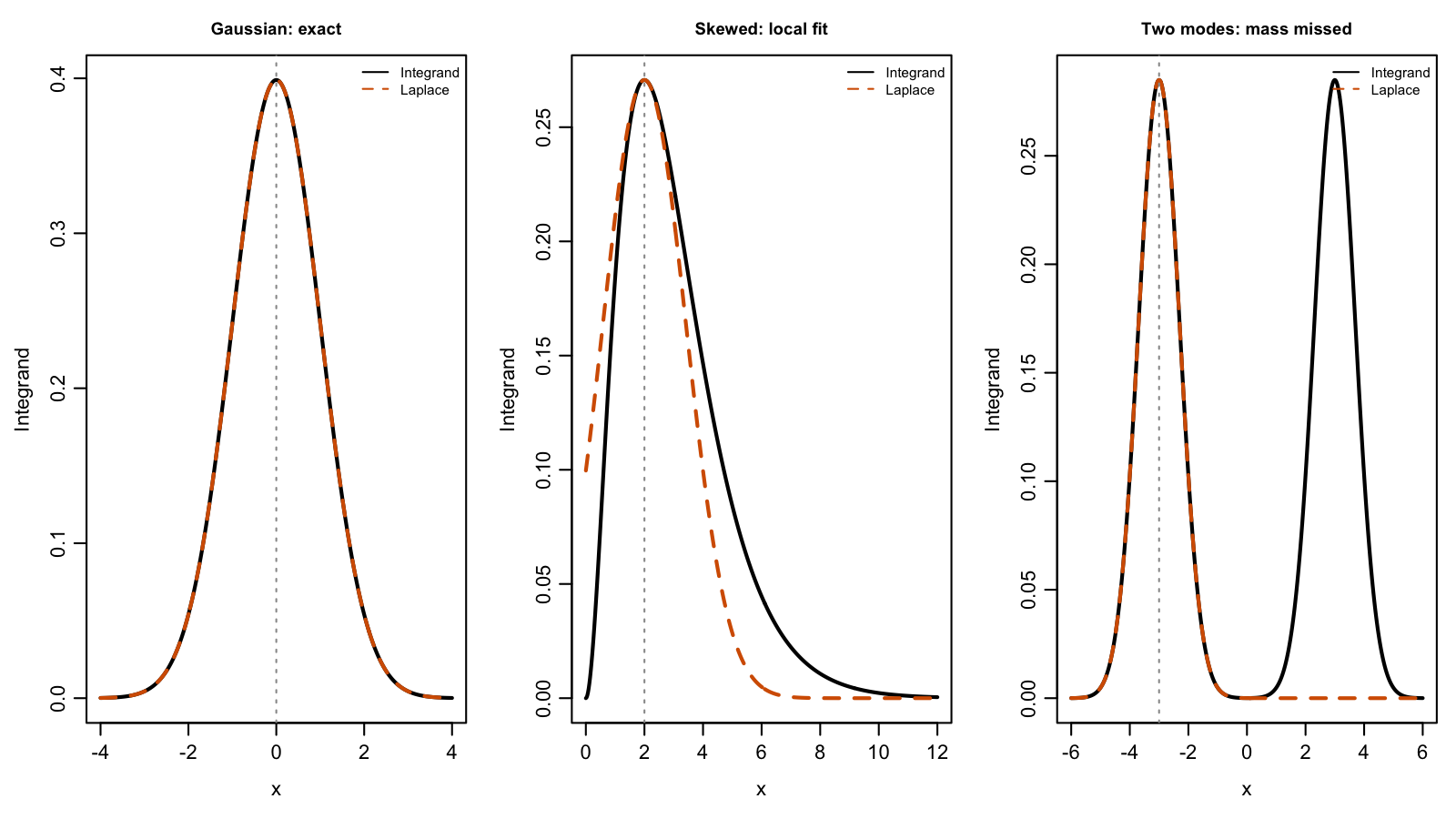
A local Gaussian fit can miss skewness or mass around another mode.
Laplace approximation: alternative version
We have \[f(y,b)=f(y)f(b\mid y).\]
Now assume \(b\mid y\) is \(N(\hat{b}_{y},H^{-1})\), and compute at \(b=\hat{b}_{y}\), \[f(y)=\frac{f(y,\hat{b}_{y})}{f(\hat{b}_{y}\mid y)}=f(y,\hat{b}_{y})\frac{(2\pi)^{d/2}}{{\rm det}(H)^{1/2}},\] since \[f(\hat{b}_{y}\mid y)=\frac{1}{(2\pi)^{d/2}{\rm det}(H)^{-1/2}}=\frac{{\rm det}(H)^{1/2}}{(2\pi)^{d/2}}.\]
So really this amounts to approximating the conditional with a Gaussian.
Monte Carlo
Something different...
Quadrature is not always appropriate. E.g.,
high-dimensional integrals
non-smooth functions.
In quadrature we compute a weighted sum \[\sum_{i=1}^{N}w_{i}f(x_{i}),\] where \(x_{i},w_{i}\) are fixed values.
A strange idea: what if we randomize the \(X_{i}\) and just use \(w_{i}=\frac{1}{N}\)?
- Surprisingly, this can be a very good idea.
Fundamental idea
The fundamental idea behind Monte Carlo integration is to view the integral of \(g\) over some set \(\mathsf{X}\) \[I=\int_{\mathsf{X}}g(x){\rm d}x,\] as the expectation of a random variable.
Find a PDF \(\pi\) such that \(\pi(x)>0\) whenever \(g(x)\neq0\), then we can write \[I=\int_{\mathsf{X}}g(x){\rm d}x=\int_{\mathsf{X}}f(x)\pi(x){\rm d}x=\mathbb{E}_{\pi}[f(X)],\] where \(f(x)=g(x)/\pi(x)\).
Idea: simulate independent \(X_{i}\sim\pi\), compute \(N^{-1}\sum_{i=1}^{N}f(X_{i})\).
Consistency, lack-of-bias
Averages of i.i.d. random variables are simple to analyze!
Consistency and unbiasedness require \(\mathbb{E}_{\pi}[|f(X)|]<\infty\): \[\frac{1}{N}\sum_{i=1}^{N}f(X_{i})\to_{p}\mathbb{E}_{\pi}[f(X)]=I.\]
Lack-of-bias: \[\mathbb{E}\left[\frac{1}{N}\sum_{i=1}^{N}f(X_{i})\right]=\mathbb{E}_{\pi}[f(X)]=I.\]
Variance, CLT
Variance: if \({\rm var}_{\pi}(f)=\mathbb{E}_{\pi}[f(X)^{2}]-\mathbb{E}_{\pi}[f(X)]^{2}<\infty\), \[{\rm var}\left(\frac{1}{N}\sum_{i=1}^{N}f(X_{i})\right)=\frac{1}{N}{\rm var}_{\pi}(f(X)).\]
CLT: \[\sqrt{N}\left\{ \frac{1}{N}\sum_{i=1}^{N}f(X_{i})-I\right\} \to_{d}N\left(0,{\rm var}_{\pi}(f)\right).\]
Quantitative control from \(\int f(x)^{2}\pi(x){\rm d}x\).
Smoothness is irrelevant.
\(L^{2}(\pi)\) is the space of finite variance functions under \(\pi\).
Simple example
Let \(I=\int_{0}^{1}x^{2}{\rm d}x\). Of course this is \(1/3\).
Let \(\pi(x)=\mathbb{I}(0<x<1)\), i.e. \(\pi\) is Uniform\((0,1)\).
Simulate \(X_{1},\ldots,X_{N}\sim\pi\) independent and compute \[\frac{1}{N}\sum_{i=1}^{N}X_{i}^{2}.\]
Variance is \[\frac{1}{N}\left[\int_{0}^{1}x^{4}{\rm d}x-\left\{ \int_{0}^{1}x^{2}{\rm d}x\right\} ^{2}\right]=\frac{1}{N}\left\{ \frac{1}{5}-\frac{1}{9}\right\} =\frac{1}{N}\cdot\frac{4}{45}.\]
What about a different \(\pi\)?
Instead, consider \(\pi(x)=2x\mathbb{I}(0<x<1)\).
Then we need \(f(x)=g(x)/\pi(x)=x^{2}/(2x)=x/2\) on \((0,1)\).
Then simulate \(X_{1},\ldots,X_{N}\sim\pi\) independent and compute \[\frac{1}{N}\sum_{i=1}^{N}\frac{X_{i}}{2}.\]
Now variance is \[\frac{1}{N}\left[\int_{0}^{1}\frac{x^{2}}{4}\,2x\,{\rm d}x-\frac{1}{9}\right]=\frac{1}{N}\left(\frac{1}{8}-\frac{1}{9}\right)=\frac{1}{72N}.\]
That’s better!
Importance sampling
If we have \(I=\int f(x)\pi(x){\rm d}x\), then importance sampling refers to the identity \[I=\int f(x)\pi(x){\rm d}x=\int f(x)w(x)\mu(x){\rm d}x,\] where \(w(x)=\pi(x)/\mu(x)\), and we assume \(\mu(x)>0\) whenever \(\pi(x)>0\).
Basically the same thing we did when coming up with \[\int g(x){\rm d}x=\int f(x)\pi(x){\rm d}x.\]
Often emphasis is on changing hard to sample \(\pi\) to easy to sample \(\mu\).
- Possibly consideration of several \(f\)’s, hence the stronger constraint.
Optimal importance distribution
Consider \(I=\int g(x){\rm d}x\).
Importance sampling variance is \[\int\left|\frac{g(x)}{\mu(x)}\right|^{2}\mu(x){\rm d}x-\left(\int g(x){\rm d}x\right)^{2},\] where the second term does not depend on \(\mu\).
Jensen’s inequality gives \[\begin{aligned}\int\frac{|g(x)|^{2}}{\mu(x)}\,{\rm d}x & \geq\left\{ \int\frac{|g(x)|}{\mu(x)}\mu(x)\,{\rm d}x\right\} ^{2}\\ & =\left\{ \int|g(x)|\,{\rm d}x\right\} ^{2}. \end{aligned}\]
Now observe that if \(\mu(x)=\left|g(x)\right|/\int\left|g(x)\right|{\rm d}x\) then \[\int\left|\frac{g(x)}{\mu(x)}\right|^{2}\mu(x){\rm d}x=\left\{ \int\left|g(x)\right|{\rm d}x\right\} ^{2},\] so this is an optimal choice!
Practical example
Often we can’t really go for optimality.
- Need to be able to actually sample according to \(\mu\).
Consider \(\pi\) the density of some complicated distribution, e.g. a Bayesian posterior density.
If we believe \(\pi\) is close to \({\rm Normal}(m,\Sigma)\), we could take \(\mu={\rm Normal}(m,\Sigma)\).
In fact, we might take for \(m\) and \(\Sigma\) the maximizer of \(\pi\) and the inverse Hessian of \(-\log\pi\) at \(m\).
- The mode must be interior and the negative log-density Hessian positive definite.
Try it in the lab...
Self-normalized importance sampling I
Try it in the lab...
Except that we often don’t know \(\pi\) precisely, but only up to a normalizing constant.
Posterior: \[\pi(\theta)=\frac{1}{Z}\pi_{0}(\theta)L(\theta;y),\] where \(Z=\int\pi_{0}(\theta)L(\theta;y){\rm d}\theta\).
We can compute unnormalized importance weights \[\tilde{w}(\theta)=L(\theta;y)\propto\cfrac{\pi(\theta)}{\pi_{0}(\theta)},\] but not \(w(\theta)\) as we can’t compute \(Z\).
Self-normalized importance sampling II
Consider general setting, \(\int f(x)\pi(x){\rm d}x\) the objective.
Imagine we can simulate from \(\mu\) with \(\tilde{w}(x)\propto\pi(x)/\mu(x)\).
Then consider the identity \[\frac{\int f(x)\tilde{w}(x)\mu(x){\rm d}x}{\int\tilde{w}(x)\mu(x){\rm d}x}=\frac{\int f(x)w(x)\mu(x){\rm d}x}{\int w(x)\mu(x){\rm d}x}=\int f(x)\pi(x){\rm d}x,\] so we can approximate numerator and denominator on LHS!
I.e., with samples \(X_{i}\sim\mu\) independent, compute \[\frac{\frac{1}{N}\sum_{i=1}^{N}\tilde{w}(X_{i})f(X_{i})}{\frac{1}{N}\sum_{i=1}^{N}\tilde{w}(X_{i})}=\frac{\sum_{i=1}^{N}\tilde{w}(X_{i})f(X_{i})}{\sum_{i=1}^{N}\tilde{w}(X_{i})}=\sum_{i=1}^{N}\bar{W}_{i}f(X_{i}),\] where the self-normalized weights are: \[\bar{W}_{i}=\frac{\tilde{w}(X_{i})}{\sum_{i=1}^{N}\tilde{w}(X_{i})}.\]
Cf. quadrature rules.
Self-normalized importance sampling III
Take independent \(X_{i}\sim\mu\), with \(\mu>0\) wherever \(\pi>0\), and \(\tilde{w}=c\pi/\mu\) for \(0<c<\infty\).
If \(\mathbb{E}_{\pi}|f(X)|<\infty\), consistency follows from the law of large numbers and a positive limiting denominator.
The estimate requires positive total sampled weight. It is generally biased.
For a CLT, require the following variance to be finite:
\[\sqrt{N}(\tilde{I}_{N}-I)\to_{d}N(0,\sigma^{2}(f)),\qquad\sigma^{2}(f)=\int(f-I)^{2}w^{2}\mu\,{\rm d}x<\infty.\]
A measure of sample quality I
One simple measure of sample quality is the so-called “effective sample size”.
It was inspired originally by quantifying the ratio of asymptotic variances with \(\mu\) and with \(\pi\).
But this is not what it actually approximates consistently...
It is (intentionally) function independent.
The effective sample size is the random variable \[\mathcal{E}_{N}=N\cdot\frac{\left\{ \frac{1}{N}\sum_{i=1}^{N}\tilde{w}(X_{i})\right\} ^{2}}{\left\{ \frac{1}{N}\sum_{i=1}^{N}\tilde{w}(X_{i})^{2}\right\} },\] with positive total weight. If the weights have finite second moment, the fraction on the right tends to \(R(\pi,\mu)=\left\{ \int w(x)^{2}\mu(x){\rm d}x\right\} ^{-1}\in(0,1]\).
The effective sample size takes values in \([1,N]\).
A measure of sample quality II
For bounded \(f\), define \(\|f\|_{{\rm osc}}=\sup f-\inf f\). Then \[\begin{align*} \sigma^{2}(f) & =\int(f(x)-I)^{2}w(x)^{2}\mu(x){\rm d}x\\ & \leq\left\Vert f\right\Vert _{{\rm osc}}^{2}\int w(x)^{2}\mu(x){\rm d}x\\ & =\frac{\left\Vert f\right\Vert _{{\rm osc}}^{2}}{R(\pi,\mu)}, \end{align*}\] The normalized ESS \(\mathcal{E}_{N}/N\) estimates the denominator \(R(\pi,\mu)\); ESS estimates \(NR(\pi,\mu)\).
We also have a relationship to the \(\chi^{2}\)-divergence between \(\pi\) and \(\mu\): \[R(\pi,\mu)=\frac{1}{1+d_{\chi^{2}}(\pi,\mu)}.\]
Proposal overlap and weight concentration
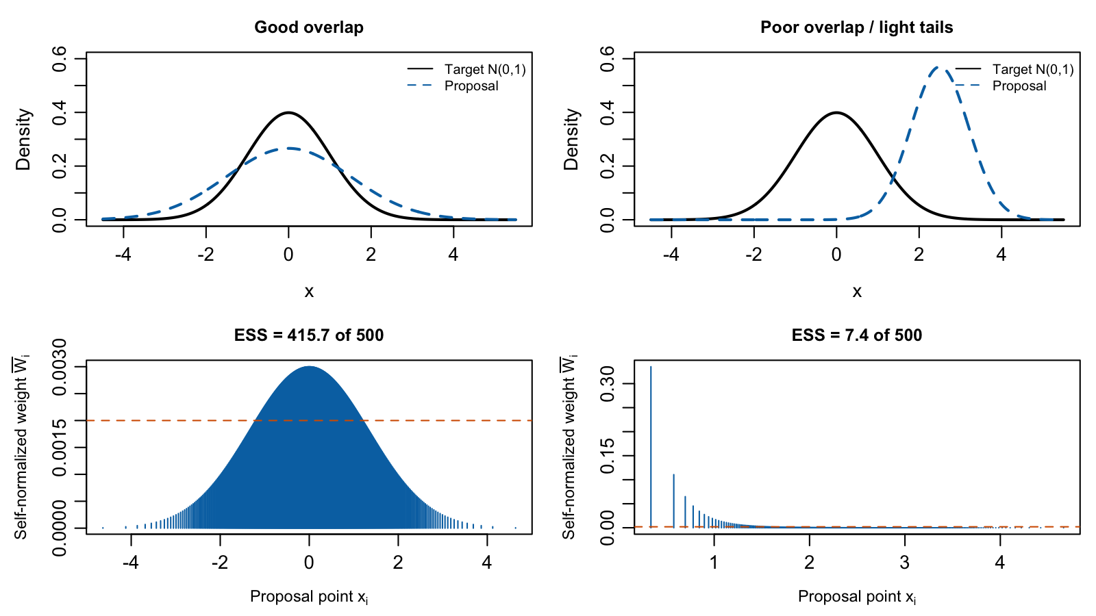
Each line shows \(\bar W_i\) at a proposal point \(x_i\): 500 fixed midpoint quantiles, rather than random draws. Dashed line: equal weights, \(1/500\). ESS alone cannot detect unvisited target mass.
Recap
Wrapping up
Low-dimensional, smooth integrands: give quadrature a go!
High-dimensional, \(L^{2}(\pi)\) functions: give Monte Carlo a go!
More seriously, these methods work for suitably simple problems, which can arise in practice.
When suitable, certainly easier to explain their use.
- Some statistical models have a lot more regularity than arbitrary functions.
For more challenging integrals, there are more advanced Monte Carlo methods.
- Markov chains, interacting particles, diffusions, auxiliary distributions, etc.