Numerical Calculus II: Integration

1 Numerical Integration

Integration is an important tool in statistics. Integration is involved in, for example:

1. integrating random effects out of a joint distribution to get a likelihood,
2. evaluating expectations, including posterior expectations in Bayesian inference.

Unfortunately integration is typically intractable and accurate approximations are often computationally expensive, so much statistical research is devoted to clever ways of avoiding it. When it can’t be avoided then the aim is typically to find ways of approximating an integral of a function with a suitably small number of function evaluations.

Integration w.r.t. 1 or 2 (maybe even up to 4) variables is not too problematic. A typical solution, often called quadrature, involves evaluating the function at a specified set of points and combining the resulting values to obtain an approximation of the integral.

In even more detail, in one dimension the idea is usually to

• split the domain into small intervals
• construct interpolating polynomials in each interval using the function evaluations
• integrate each interpolating polynomial over each interval
• sum the values together.

At least in principle, one can then approximate higher dimensional integrals by viewing them as iterated one-dimensional integrals. This is only practical for a small number of dimensions as the cost grows exponentially with dimension.

For higher-dimensional problems, which occur frequently in Statistics, we often resort to random algorithms that do not always scale so poorly with dimension.

2 Quadrature

To focus on the main ideas, we will restrict our attention to numerically approximating the definite integral of a function \(f\) over a finite interval \([a,b]\). Extensions to semi-infinite and infinite intervals will be discussed briefly, as will extensions to multiple integrals.

In practice, for one dimensional integrals you can use R’s integrate function. For multiple integrals, the cubature package can be used. Unlike the basics covered here, these functions will produce error estimates and should be more robust.

2.1 Polynomial interpolation

We consider approximation of a continuous function \(f\) on \([a,b]\), i.e. \(f \in C^0([a,b])\) using a polynomial function \(p\). One practical motivation is that polynomials can be integrated exactly.

One way to devise an approximation is to first consider approximating \(f\) using an interpolating polynomial with, say, \(k\) points \(\{(x_i,f(x_i))\}_{i=1}^k\). The interpolating polynomial is unique, has degree at most \(k-1\), and it is convenient to express it as a Lagrange polynomial:

\[p_{k-1}(x) := \sum_{i=1}^k \ell_i(x) f(x_i),\]

where the Lagrange basis polynomials are

\[\ell_i(x) = \prod_{j=1,j\neq i}^k \frac{x-x_j}{x_i-x_j} \qquad i \in \{1,\ldots,k\}.\] For a given 3rd degree polynomial \(f\), we plot polynomial approximations for \(k \in \{2,3,4\}\) and specific choices of \(x_1,\ldots,x_4\).

construct.interpolating.polynomial <- function(f, xs) {
  k <- length(xs)
  fxs <- f(xs)
  p <- function(x) {
    value <- 0
    for (i in 1:k) {
      fi <- fxs[i]
      zs <- xs[setdiff(1:k,i)]
      li <- prod((x-zs)/(xs[i]-zs))
      value <- value + fi*li
    }
    return(value)
  }
  return(p)
}

plot.polynomial.approximation <- function(f, xs, a, b) {
  p <- construct.interpolating.polynomial(f, xs)
  vs <- seq(a, b, length.out=500)
  plot(vs, f(vs), type='l', xlab="x", ylab="black: f(x), red: p(x)")
  points(xs, f(xs), pch=20)
  lines(vs, vapply(vs, p, 0), col="red")
}

a <- -4
b <- 4

f <- function(x) {
  return(-x^3 + 3*x^2 - 4*x + 1)
}

plot.polynomial.approximation(f, c(-2, 2), a, b)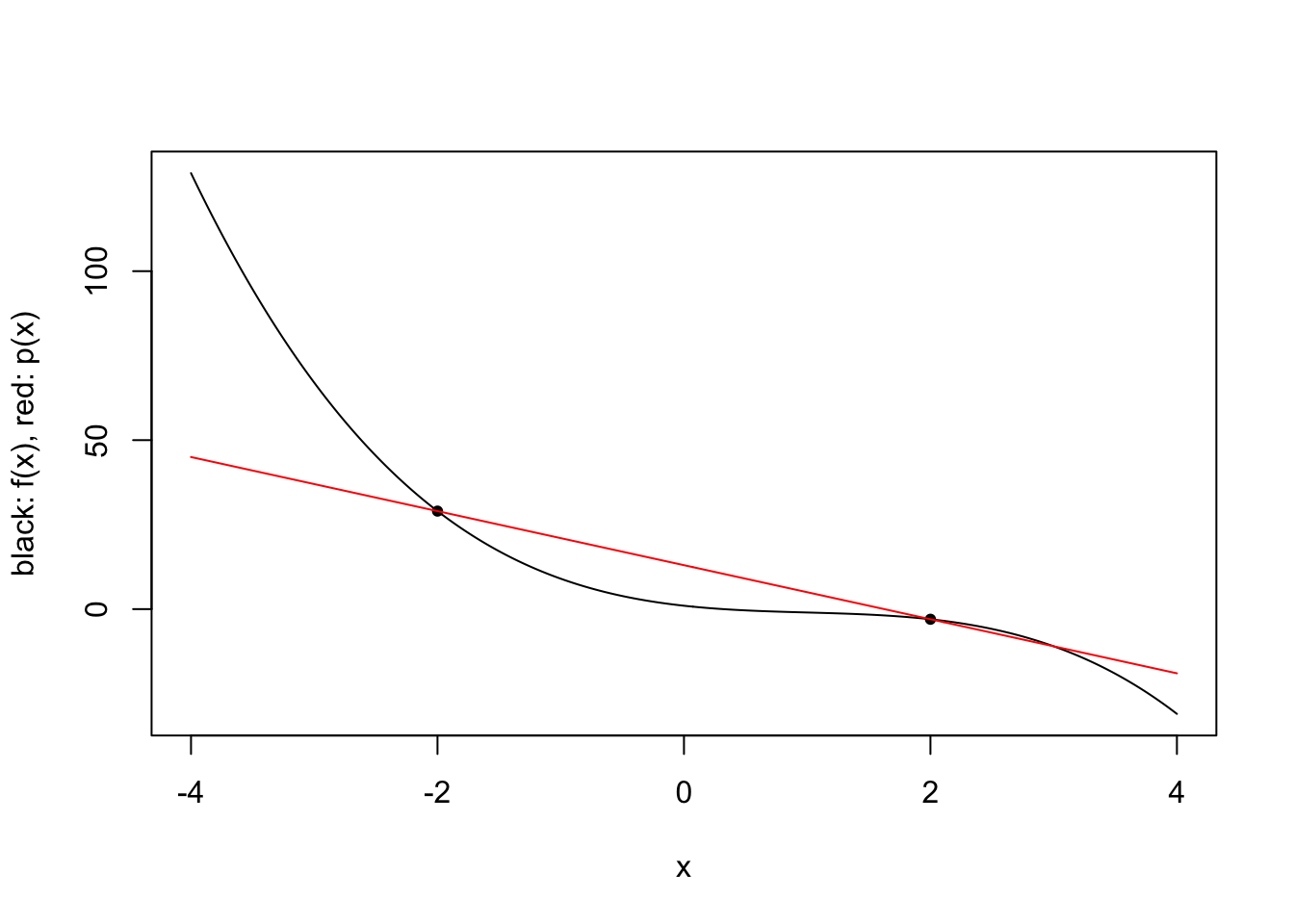

plot.polynomial.approximation(f, c(-2, 0, 2), a, b)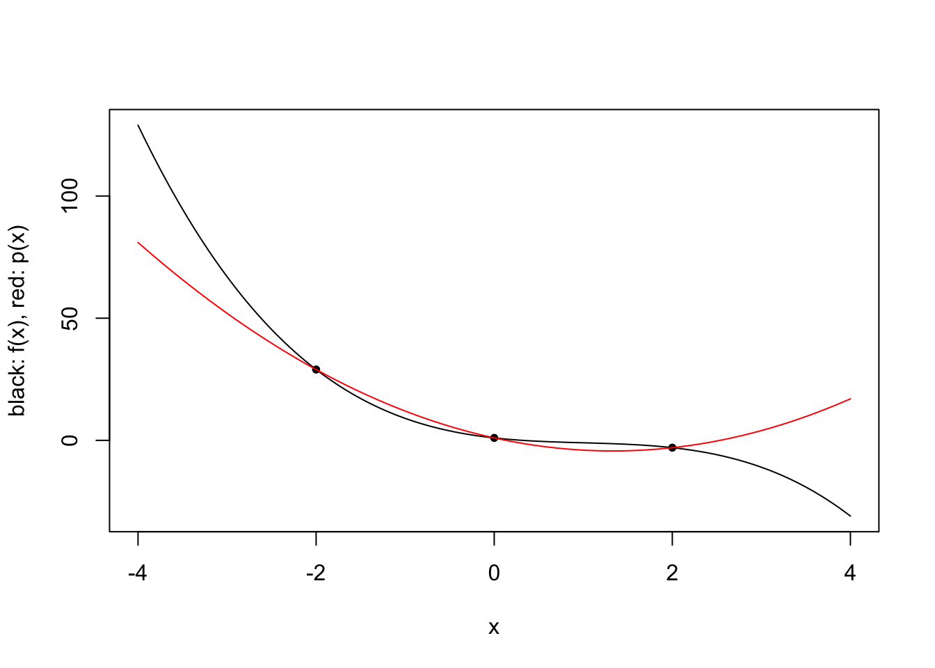

plot.polynomial.approximation(f, c(-2, 0, 2, 4), a, b)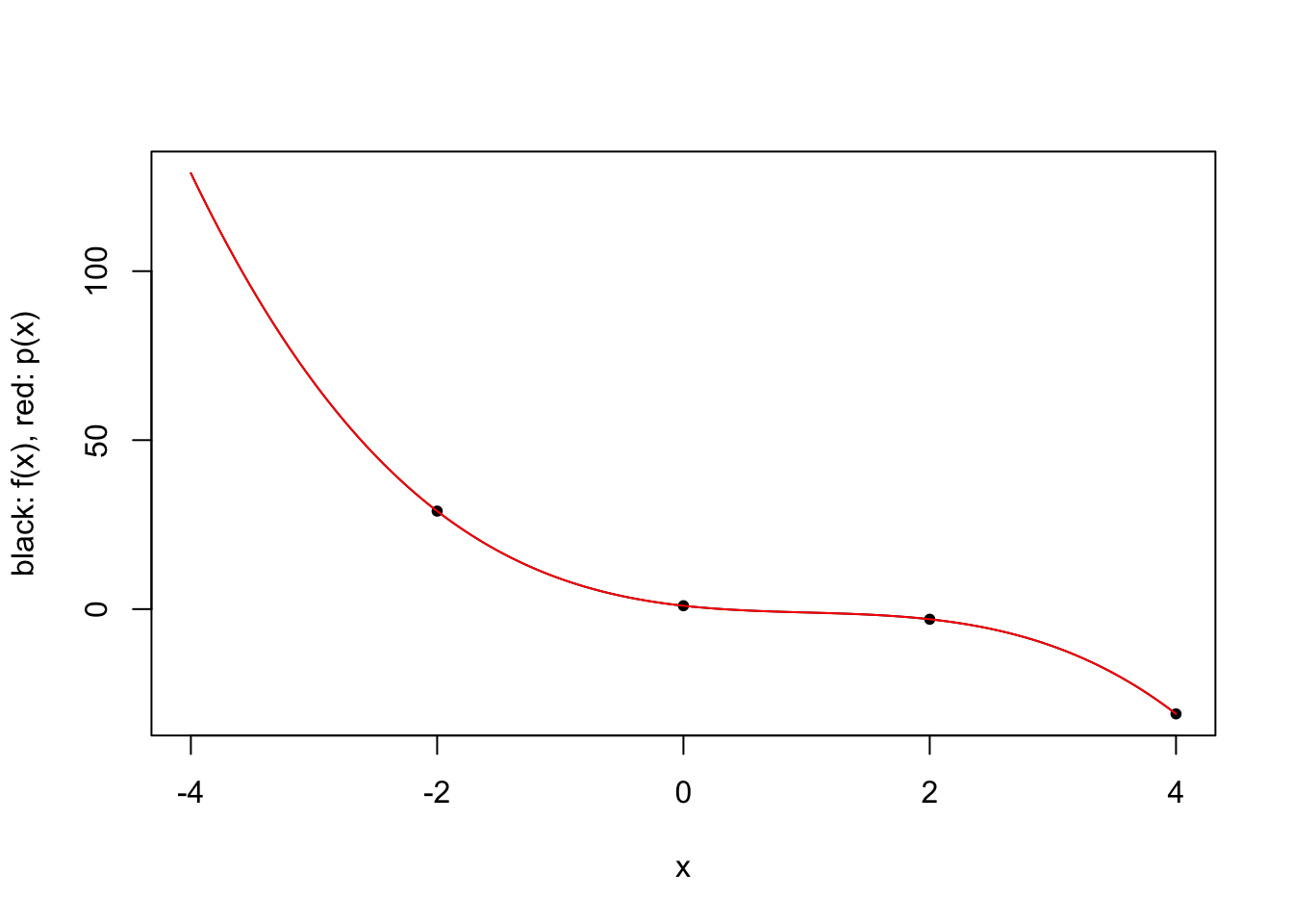

Of course, one might instead want a different representation of the polynomial, e.g. as sums of monomials with appropriate coefficients.

\[p(x) = \sum_{i=1}^k a_i x^{i-1}.\]

This can be accomplished in principle by solving a linear system. In practice, this representation is often avoided for large \(k\) as solving the linear system is numerically unstable.

An alternative to using many interpolation points to fit a high-degree polynomial is to approximate the function with different polynomials in a number of subintervals of the domain. This results in a piecewise polynomial approximation that is not necessarily continuous.

We consider a simple scheme where \([a,b]\) is partitioned into a number of equal length subintervals, and within each subinterval \(k\) interpolation points are used to define an approximating polynomial. To keep things simple, we consider only two possible ways to specify the \(k\) interpolation points within each subinterval. In both cases the points are evenly spaced and evenly spaced from the endpoints of the interval. However, when the scheme is “closed”, the endpoints of the interval are included, while when the scheme is “open”, the endpoints are not included. For a closed scheme with \(k=1\), we opt to include the left endpoint.

# get the endpoints of the subintervals
get.subinterval.points <- function(a, b, nintervals) {
  return(seq(a, b, length.out=nintervals+1))
}

# returns which subinterval a point x is in
get.subinterval <- function(x, a, b, nintervals) {
  h <- (b-a)/nintervals
  return(min(max(1,ceiling((x-a)/h)),nintervals))
}

# get the k interpolation points in the interval
# this depends on the whether the scheme is open or closed
get.within.subinterval.points <- function(a, b, k, closed) {
  if (closed) {
    return(seq(a, b, length.out=k))
  } else {
    h <- (b-a)/(k+1)
    return(seq(a+h,b-h,h))
  }
}

construct.piecewise.polynomial.approximation <- function(f, a, b, nintervals, k, closed) {
  ps <- vector("list", nintervals)
  subinterval.points <- get.subinterval.points(a, b, nintervals)
  for (i in 1:nintervals) {
    left <- subinterval.points[i]
    right <- subinterval.points[i+1]
    points <- get.within.subinterval.points(left, right, k, closed)
    p <- construct.interpolating.polynomial(f, points)
    ps[[i]] <- p
  }
  p <- function(x) {
    return(ps[[get.subinterval(x, a, b, nintervals)]](x))
  }
  return(p)
}

plot.piecewise.polynomial.approximation <- function(f, a, b, nintervals, k, closed) {
  p <- construct.piecewise.polynomial.approximation(f, a, b, nintervals, k, closed)
  vs <- seq(a, b, length.out=500)
  plot(vs, f(vs), type='l', xlab="x", ylab="black: f(x), red: p(x)")
  lines(vs, vapply(vs, p, 0), col="red")
  subinterval.points <- get.subinterval.points(a, b, nintervals)
  for (i in 1:nintervals) {
    left <- subinterval.points[i]
    right <- subinterval.points[i+1]
    pts <- get.within.subinterval.points(left, right, k, closed)
    points(pts, f(pts), pch=20, col="blue")
  }
  abline(v = subinterval.points)
}

plot.piecewise.polynomial.approximation(sin, 0, 10, 5, 1, TRUE)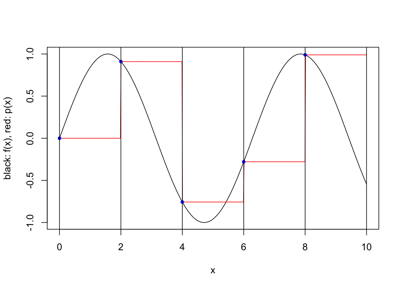

plot.piecewise.polynomial.approximation(sin, 0, 10, 5, 2, TRUE)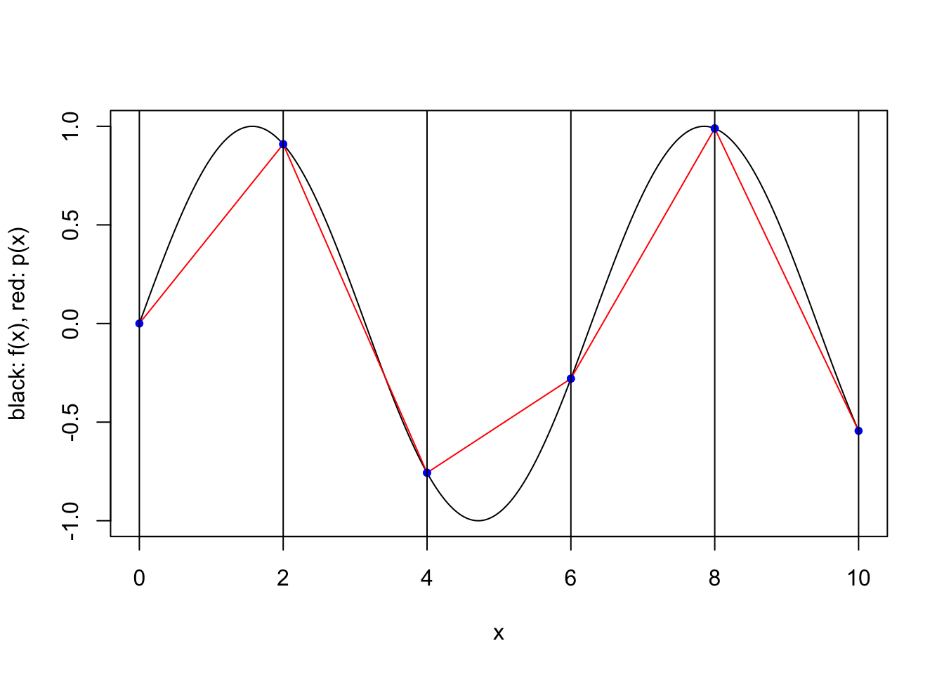

plot.piecewise.polynomial.approximation(sin, 0, 10, 5, 2, FALSE)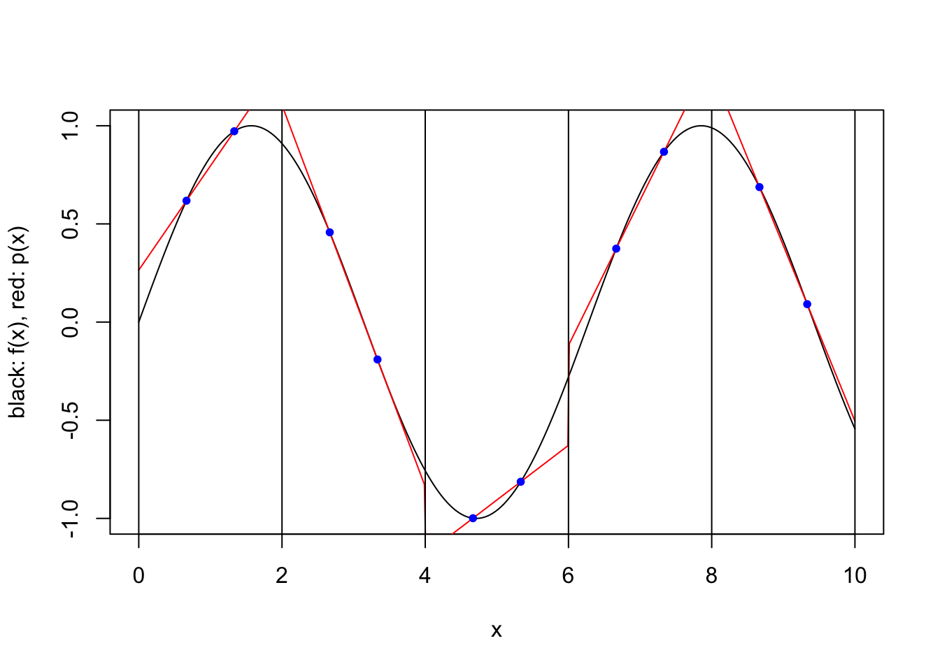

plot.piecewise.polynomial.approximation(sin, 0, 10, 5, 3, TRUE)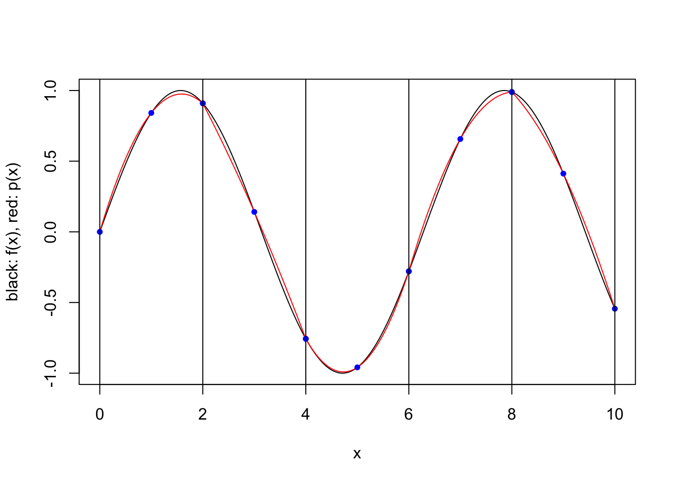

plot.piecewise.polynomial.approximation(sin, 0, 10, 20, 1, TRUE)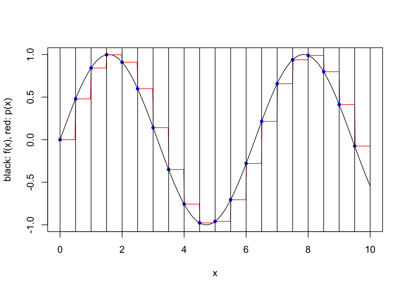

plot.piecewise.polynomial.approximation(sin, 0, 10, 20, 1, FALSE)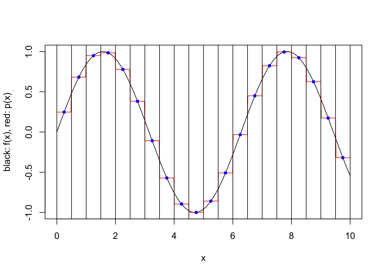

2.2 Polynomial integration

We now consider approximating the integral

\[I(f) := \int_a^b f(x) {\rm d}x,\]

where \(f \in C^0([a,b])\).

All of the approximations we will consider here involve computing integrals associated with the polynomial approximations. The approximations themselves are often referred to as quadrature rules.

2.2.1 Changing the limits of integration

For constants \(a<b\) and \(c<d\), we can accommodate a change of finite interval via

\[\int_a^b f(x) {\rm d}x = \int_c^d g(y) {\rm d}y,\]

by defining

\[g(y) := \frac{b-a}{d-c} f \left (a+\frac{b-a}{d-c}(y-c) \right ).\]

Examples of common intervals are \([-1,1]\) and \([0,1]\).

change.domain <- function(f, a, b, c, d) {
  g <- function(y) {
    return((b-a)/(d-c)*f(a + (b-a)/(d-c)*(y-c)))
  }
  return(g)
}

# test out the function using R's integrate function
integrate(sin, 0, 10)

1.839072 with absolute error < 9.9e-12

g = change.domain(sin, 0, 10, -1, 1)
integrate(g, -1, 1)

1.839072 with absolute error < 9.9e-12

One can also accommodate a semi-infinite interval by a similar change of variables. One example is

\[\int_a^\infty f(x) {\rm d}x = \int_0^1 g(y) {\rm d}y, \qquad g(y) := \frac{1}{(1-y)^2} f \left ( a + \frac{y}{1-y} \right ).\]

Similarly, one can transform an integral over \(\mathbb{R}\) to one over \([-1,1]\)

\[\int_{-\infty}^\infty f(x) {\rm d}x = \int_{-1}^1 g(t) {\rm d}t, \qquad g(t) := \frac{1+t^2}{(1-t^2)^2} f \left ( \frac{t}{1-t^2} \right ).\]

We will only consider finite intervals here.

2.2.2 Integrating the interpolating polynomial approximation

Consider integrating a Lagrange polynomial \(p_{k-1}\) over \([a,b]\). We have \[\begin{align} I(p_{k-1}) &= \int_a^b p_{k-1}(x) {\rm d}x \\ &= \int_a^b \sum_{i=1}^k \ell_i(x) f(x_i) {\rm d}x \\ &= \sum_{i=1}^k f(x_i) \int_a^b \ell_i(x) {\rm d}x \\ &= \sum_{i=1}^k w_i f(x_i), \end{align}\] where for \(i \in \{1,\ldots,k\}\), \(w_i := \int_a^b \ell_i(x) {\rm d}x\) and we recall that \(\ell_i(x) = \prod_{j=1,j\neq i}^k \frac{x-x_j}{x_i-x_j}\).

The approximation of \(I(f)\) is \(\hat{I}(f) = I(p_{k-1})\), where \(p_{k-1}\) depends only on the choice of interpolating points \(x_1,\ldots,x_k\).

The functions \(\ell_i\) can be a bit complicated, but certainly can be integrated by hand quite easily for small values of \(k\). For example, with \(k=1\) we have \(\ell_1 \equiv 1\), so the integral \(\int_a^b \ell_1(x) {\rm d}x = b-a\). For \(k=2\) we have \(\ell_1(x) = (x-x_2)/(x_1-x_2)\), yielding \[\int_a^b \ell_1(x) {\rm d}x = \frac{b-a}{2(x_1-x_2)}(b+a-2x_2),\] and similarly \(\ell_2(x) = (x-x_1)/(x_2-x_1)\), so \[\int_a^b \ell_2(x) {\rm d}x = \frac{b-a}{2(x_2-x_1)}(b+a-2x_1).\]

2.3 Newton–Cotes rules

The rectangular rule corresponds to a closed scheme with \(k=1\):

\[\hat{I}_{\rm rectangular}(f) = (b-a) f(a).\]

The midpoint rule corresponds to an open scheme with \(k=1\):

\[\hat{I}_{\rm midpoint}(f) = (b-a) f \left ( \frac{a+b}{2} \right).\]

The trapezoidal rule corresponds to a closed scheme with \(k=2\). Since \((x_1,x_2) = (a,b)\), we obtain \(\int_a^b \ell_1(x) {\rm d}x = (b-a)/2\) and

\[\hat{I}_{\rm trapezoidal}(f) = \frac{b-a}{2} \{ f(a)+f(b) \}.\]

Simpson’s rule corresponds to a closed scheme with \(k=3\). After some calculations, we obtain

\[\hat{I}_{\rm Simpson}(f) = \frac{b-a}{6} \left \{ f(a) + 4 f \left ( \frac{a+b}{2} \right) + f(b) \right \}.\]

We can obtain bounds on the error of integration using any sequence of interpolation points, for sufficiently smooth functions.

rule	\(\hat{I}(f) - I(f)\), with \(\xi \in (a,b)\)
rectangular	\(-\frac{1}{2}(b-a)^2 f'(\xi)\)
midpoint	\(-\frac{1}{24}(b-a)^3 f^{(2)}(\xi)\)
trapezoidal	\(\frac{1}{12}(b-a)^3 f^{(2)}(\xi)\)
Simpson	\(\frac{1}{2880}(b-a)^5 f^{(4)}(\xi)\)

This indicates that the midpoint rule, which uses only one point, is often better than the trapezoidal rule, which uses 2. These are both significantly worse than Simpson’s rule, which uses 3 points. One might think that using large numbers of points is beneficial, but this is not always the case since the interpolating polynomial may become quite poor when using equally spaced points as seen before. We also see that the rectangular and trapezoidal rules are exact for constant functions, the midpoint rule is exact for linear functions, and Simpson’s rule is exact for polynomials of degree up to 3.

newton.cotes <- function(f, a, b, k, closed) {
  if (k == 1) {
    if (closed) {
      return((b-a)*f(a))
    } else {
      return((b-a)*f((a+b)/2))
    }
  }
  if (k == 2 && closed) {
    return((b-a)/2*(f(a)+f(b)))
  }
  if (k == 3 && closed) {
    return((b-a)/6*(f(a)+4*f((a+b)/2)+f(b)))
  }
  stop("not implemented")
}

nc.example <- function(f, name, value) {
  df <- data.frame(f=character(), rule=character(), error=numeric())
  df <- rbind(df, data.frame(f=name, rule="Rectangular", error=newton.cotes(f,0,1,1,TRUE)-value))
  df <- rbind(df, data.frame(f=name, rule="Midpoint", error=newton.cotes(f,0,1,1,FALSE)-value))
  df <- rbind(df, data.frame(f=name, rule="Trapezoidal", error=newton.cotes(f,0,1,2,TRUE)-value))
  df <- rbind(df, data.frame(f=name, rule="Simpson's", error=newton.cotes(f,0,1,3,TRUE)-value))
  return(df)
}

df <- nc.example(function(x) x, "x", 1/2)
df <- rbind(df, nc.example(function(x) x^2, "x^2", 1/3))
df <- rbind(df, nc.example(function(x) x^3, "x^3", 1/4))
df <- rbind(df, nc.example(function(x) x^4, "x^4", 1/5))

ggplot(df, aes(fill=rule, y=error, x=f)) + geom_bar(position="dodge", stat="identity")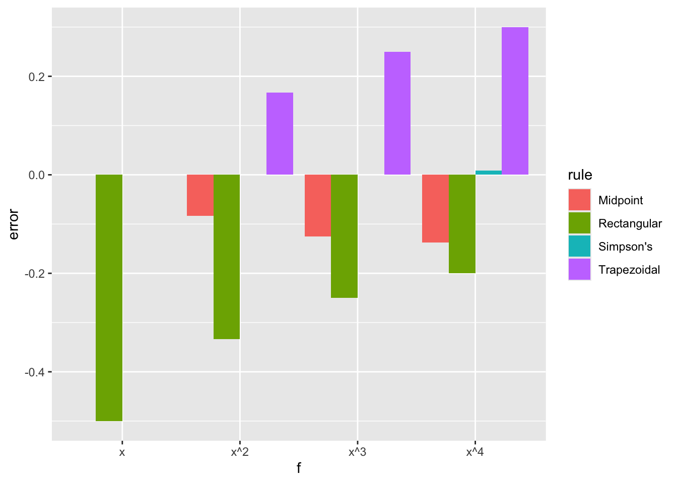

2.3.1 Composite rules

When a composite polynomial interpolation approximation is used, the integral of the approximation is simply the sum of the integrals associated with each subinterval. Hence, a composite Newton–Cotes rule is obtained by splitting the interval \([a,b]\) into \(m\) subintervals and summing the approximate integrals from the Newton–Cotes rule for each subinterval. \[\hat{I}^m_{\rm rule}(f) = \sum_{i=1}^m \hat{I}_{\rm rule}(f_i),\] where \(f_i\) is \(f\) restricted to \([a+(i-1)h, a+ih]\) and \(h=(b-a)/m\).

composite.rule <- function(f, a, b, subintervals, rule) {
  subinterval.points <- get.subinterval.points(a, b, subintervals)
  s <- 0
  for (i in 1:subintervals) {
    left <- subinterval.points[i]
    right <- subinterval.points[i+1]
    s <- s + rule(f, left, right)
  }
  return(s)
}

# composite Newton--Cotes
composite.nc <- function(f, a, b, subintervals, k, closed) {
  rule <- function(f, left, right) {
    newton.cotes(f, left, right, k, closed)
  }
  return(composite.rule(f, a, b, subintervals, rule))
}

We obtain the following composite errors, in which the dependence on \(m\) is of particular interest.

rule	\(\hat{I}^m(f) - I(f)\), with \(\xi \in (a,b)\)
rectangular	\(-\frac{1}{2m}(b-a)^2 f'(\xi)\)
midpoint	\(-\frac{1}{24m^2}(b-a)^3 f^{(2)}(\xi)\)
trapezoidal	\(\frac{1}{12m^2}(b-a)^3 f^{(2)}(\xi)\)
Simpson	\(\frac{1}{2880m^4}(b-a)^5 f^{(4)}(\xi)\)

We plot the errors against their theoretical values for \(f = \sin\), \((a,b) = (0,10)\) and different numbers of subintervals, \(m\). We replace \(f^{(s)}(\xi)\) in the theoretical expression with \((b-a)^{-1} \int_a^b f^{(s)}(x) {\rm d}x\), which should be accurate for large values of \(m\).

ms <- c(10:19, seq(20, 500, 10))

composite.rectangular <- vapply(ms, function(m) composite.nc(sin, 0, 10, m, 1, TRUE), 0)

composite.midpoints <- vapply(ms, function(m) composite.nc(sin, 0, 10, m, 1, FALSE), 0)

composite.trapezoidal <- vapply(ms, function(m) composite.nc(sin, 0, 10, m, 2, TRUE), 0)

composite.simpsons <- vapply(ms, function(m) composite.nc(sin, 0, 10, m, 3, TRUE), 0)

val <- 1-cos(10) # integral of sin(x) for x=0..10
v1 <- -sin(10)/10 # integral of sin'(x)/10 for x=0..10
v2 <- val/10 # integral of sin(x)/10 for x=0..10

tr <- tibble(m=ms, rule="rectangular", log.error=log(composite.rectangular - val),
             theory=log(v1*1/2*10^2/ms))
tt <- tibble(m=ms, rule="trapezoidal", log.error=log(val - composite.trapezoidal),
             theory=log(v2*1/12*10^3/ms^2))
tm <- tibble(m=ms, rule="midpoints", log.error=log(composite.midpoints - val),
            theory=log(v2*1/24*10^3/ms^2))
ts <- tibble(m=ms, rule="simpsons", log.error=log(composite.simpsons - val),
            theory=log(v2*1/2880*10^5/ms^4))
tib <- bind_rows(tr, tt, tm, ts)
ggplot(tib, aes(x=m, colour=rule)) + geom_point(aes(y=log.error)) + geom_line(aes(y=theory))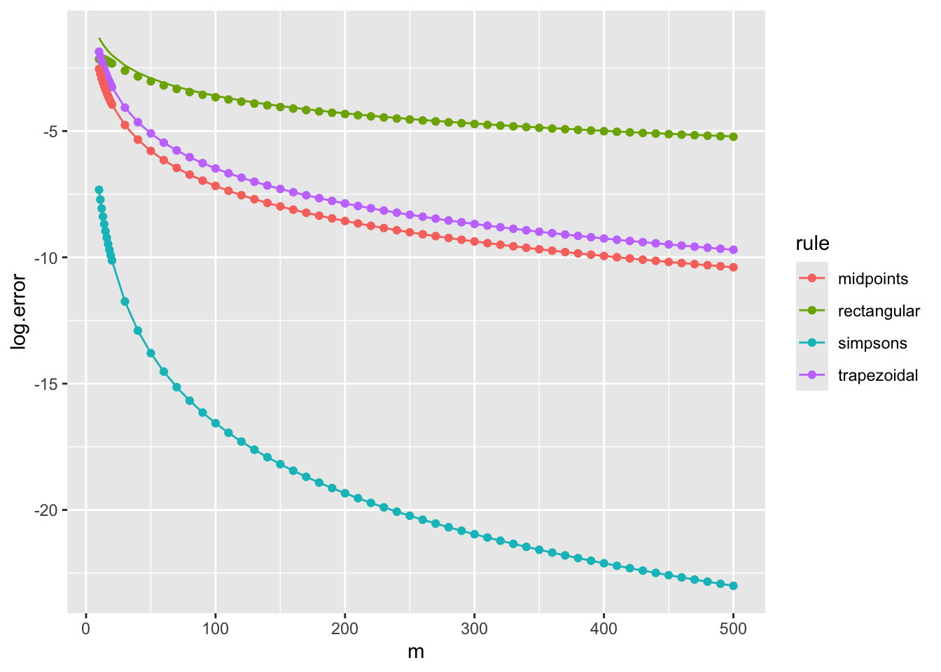

2.4 Gaussian quadrature

So far we have considered fairly simple choices for the interpolation points. In fact, one can use some nice mathematics involving orthogonal polynomials to show that choosing a special set of points will improve the approximation accuracy for the polynomial integral approximations, even when the interpolating polynomial is not that close to the true function. See https://awllee.github.io/sc1/integration/quadrature/#gaussian-quadrature for details.

The R package statmod has a nice gauss.quad function for producing the weights, \(w_i\) and nodes, \(x_i\), for some standard families of orthogonal polynomials. It assumes \(a=-1\), \(b=1\), but we can just linearly re-scale our actual interval to use this. Here is an example approximating \[\int_0^{5} \exp(x) {\rm d}x,\] with Gaussian quadrature.

library(statmod)
N <- 4
gq <- gauss.quad(N) # get the x_i, w_i
gq # take a look

$nodes
[1] -0.8611363 -0.3399810  0.3399810  0.8611363

$weights
[1] 0.3478548 0.6521452 0.6521452 0.3478548

g <- change.domain(exp, 0, 5, -1, 1)
sum(gq$weights*g(gq$nodes))

[1] 147.3976

integrate(exp,0,5)

147.4132 with absolute error < 1.6e-12

We see that using only 4 points is sufficient to get a reasonably good approximation.

One often uses composite schemes with Gaussian quadrature within each subinterval.

2.5 Multiple integrals

We have seen that one-dimensional integrals of sufficiently smooth functions on a finite domain \([a,b]\) can be approximated to arbitrary accuracy with relatively small computational cost. We consider now only a very simple approach to multiple integrals. Consider an integral over \(D = [a_1,b_1] \times \cdots \times [a_d,b_d]\).

\[I(f) = \int_D f(x_1,\ldots,x_d) {\rm d}(x_1,\ldots,x_d).\]

Appealing to Fubini’s Theorem, and letting \(D' = [a_2,b_2] \times \cdots \times [a_d,b_d]\) we can often rewrite \(I(f)\) as an iterated integral

\[I(f) = \int_{a_1}^{b_1} \int_{D'} f(x_1,\ldots,x_d) {\rm d}(x_2,\ldots,x_d) {\rm d}x_1 = \int_{a_1}^{b_1} g(x_1) {\rm d}x_1,\] where taking \(h_{x_1}(x_2,\ldots,x_d) = f(x_1,\ldots,x_d)\) we have \[g(x_1) = I(h_{x_1}) = \int_{D'} h_{x_1}(x_2,\ldots,x_d) {\rm d}(x_2,\ldots,x_d).\]

2.5.1 Recursive algorithm

It is natural to define a recursive algorithm whereby one uses an approximation of \(g\) obtained by numerical integration to approximate \(I(f)\). That is, we use the one-dimensional quadrature rule

\[\hat{I}(f) = \sum_{i=1}^k \hat{g}(x_1^{(i)}) \int_{a_1}^{b_1} \ell_i(x_1) {\rm d}x_1,\]

where \(\hat{g}(x_1) = \hat{I}(h_{x_1})\).

We implement this recursive algorithm in R, using the Gauss–Legendre (k=5) rule for every one-dimensional integral.

# approximates multiple integrals using nested composite Simpson's
# f should take a vector of length d as input, and as and bs should be the lower
# and upper limits of integration
my.integrate <- function(f, as, bs, subintervals) {
  stopifnot(length(as) == length(bs))
  d <- length(as) # dimension is length of limit vectors
  if (d == 1) {
    # just integrate the 1D function using Simpson's rule
    return(composite.nc(f, as, bs, subintervals, 3, TRUE))
  } else {
    # define a 1D function obtained by (approximately) integrating x_2,...,x_d
    g.hat <- function(x) {
      my.integrate(function(y) f(c(x,y)), as[2:d], bs[2:d], subintervals)
    }
    # integrate g.hat
    return(composite.nc(g.hat, as[1], bs[1], subintervals, 3, TRUE))
  }
}

We can test out the algorithm on a slightly challenging three-dimensional integral. Specifically, the \(\sin\) function cannot be approximated well by a degree 9 polynomial over \([0, 8\pi + 3\pi/2]\), so a few subintervals are required to give accurate answers.

f <- function(x) {
  sin(sum(x))
}

# actual value is 2
vapply(1:25, function(m) my.integrate(f, rep(0,3), rep(8*pi+3*pi/2,3), m), 0)

 [1] 1504.629751  527.788215 -116.585866  -35.786550  533.619950    8.874459
 [7]    3.739610    2.741849    2.390426    2.230713    2.146977    2.098801
[13]    2.069186    2.050044    2.037170    2.028227    2.021844    2.017183
[19]    2.013710    2.011078    2.009052    2.007471    2.006223    2.005226
[25]    2.004421

2.5.2 The curse of dimensionality

As in the one-dimensional case, numerical integration via polynomial interpolation can in principle provide very accurate approximations for sufficiently smooth functions. However, the computational cost of the algorithm grows rapidly with dimension.

Although we have defined the multiple integral algorithm recursively, to take advantage of existing functions, one can also see that its multiple integral, or “cubature”, rule is of the form \[\hat{I}(f) = \sum_{i=1}^{n} w_i f(x_i),\] where the points \(x_1,\ldots,x_n\) are arranged in \(d\)-dimensional space. The my.integrate function arranges \(n = (mk)^d\) points in a regular grid. One can clearly see that for fixed \((m,k)\), the computational cost is exponential in \(d\) and so quickly becomes prohibitive as \(d\) increases.

One may wonder if the curse of dimensionality is specific to regular grids, as indeed there are better rules that use irregular grids. However, there are certainly classes of functions that require exponential in \(d\) computational time; see, e.g. a recent survey of complexity results.

It is clear that the smoothness of \(f\) is important for the quadrature rules that we have considered. From the survey linked above, we can see that for \(r \in \mathbb{N}\), the class of \(C^r([0,1]^d)\) functions with all partial derivatives bounded by 1 does suffer from the curse. However, an outstanding open problem is whether the class of \(C^\infty([0,1]^d)\) functions with all partial derivatives bounded by 1 suffers from the curse. For a smaller class of infinitely differentiable functions, the curse does not hold. See also this recent paper for some recent progress on integration schemes with optimal convergence rates.

When one requires an approximation of a high-dimensional integral in many statistical applications, one often resorts to Monte Carlo methods as they do not suffer from the curse of dimensionality in the same way as the quadrature rules we have seen here.

3 Approximating the integrand

Beyond a few dimensions, quadrature rules really run out of steam. In statistical work, where we are often interested in integrating probability density functions, or related quantities, it is sometimes possible to approximate the integrand by a function with a known integral. Here, just one approach will be illustrated: Laplace approximation. The typical application of the method is when we have a joint density \(f({\bf y},{\bf b})\) and want to evaluate the marginal p.d.f. of \(\bf y\), \[ f_y({\bf y}) = \int f({\bf y},{\bf b}) d{\bf b}. \] For a given \(\bf y\) let \(\hat {\bf b}_y\) be the value of \(\bf b\) maximising \(f\). Then Taylor’s theorem implies that \[ \log \{f({\bf y},{\bf b}) \} \simeq \log \{f({\bf y},\hat {\bf b}_y) \} - \frac{1}{2} ({\bf b } - \hat {\bf b}_y)^{\sf T}{\bf H} ({\bf b } - \hat {\bf b}_y) \] where \(\bf H\) is the Hessian of \(-\log (f)\) w.r.t. \(\bf b\) evaluated at \({\bf y}, \hat {\bf b}_y\). i.e. \[ f({\bf y},{\bf b}) \simeq f({\bf y},\hat {\bf b}_y) \exp \left \{ - \frac{1}{2} ({\bf b } - \hat {\bf b}_y)^{\sf T}{\bf H} ({\bf b } - \hat {\bf b}_y) \right \} \] and so \[ f_y({\bf y}) \simeq f({\bf y},\hat {\bf b}_y) \int \exp \left \{ - \frac{1}{2} ({\bf b } - \hat {\bf b}_y)^{\sf T}{\bf H} ({\bf b } - \hat {\bf b}_y) \right \} d{\bf b}. \] From the properties of normal p.d.f.s we have \[ \int \frac{|{\bf H}|^{1/2}}{(2 \pi)^{d/2}} e^{ - \frac{1}{2} ({\bf b } - \hat {\bf b}_y)^{\sf T}{\bf H} ({\bf b } - \hat {\bf b}_y)} d{\bf b} =1 \Rightarrow \int e^{ - \frac{1}{2} ({\bf b } - \hat {\bf b}_y)^{\sf T}{\bf H} ({\bf b } - \hat {\bf b}_y) } d{\bf b} = \frac{(2 \pi)^{d/2}}{|{\bf H}|^{1/2}} \] so \[ f_y({\bf y}) \simeq f({\bf y},\hat {\bf b}_y) \frac{(2 \pi)^{d/2}}{|{\bf H}|^{1/2}}. \] Notice that the basic ingredients of this approximation are the Hessian of the log integrand w.r.t \({\bf b}\) and the \(\hat {\bf b}_y\) values. Calculating the latter is an optimization problem, which can usually be solved by a Newton type method, given that we can presumably obtain gradients as well as the Hessian. The highest cost here is the Hessian calculation, which scales with the square of the dimension, at worst, or for cheap integrands the determinant evaluation, which scales as the cube of the dimension. i.e. when it works, this approach is much cheaper than brute force quadrature.

4 Monte Carlo integration

The fundamental idea behind Monte Carlo integration is to view the integral of \(g\) over some set \(\mathsf{X}\) \[I=\int_{\mathsf X} g(x) {\rm d}x,\] as the expectation of a random variable. That is, if we find a probability density function (PDF) \(\pi\) such that \(\pi(x) > 0\) whenever \(g(x) \neq 0\), then we can write \[I=\int_{\mathsf X} g(x) {\rm d}x = \int_{\mathsf X} f(x) \pi(x){\rm d}x = \mathbb{E}_\pi[f(X)],\] where \(f(x) = g(x)/\pi(x)\). One can think of \(Y = f(X)\), where \(X \sim \pi\) as a random variable.

This leads naturally to algorithms for approximating \(I\) when we can simulate realizations of \(X \sim \pi\) on a computer.

Naturally, all of the simple things we know about averages of independent and identically distributed random variables can then be used fruitfully to analyze a Monte Carlo approximation of the integral: \[\hat{I}_N = \frac{1}{N}\sum_{i=1}^{N}f(X_i).\] The sequence of approximations converges in probability (and almost surely) to \(I\) as \(N \to \infty\).

Moreover, \(\mathbb{E}(\hat{I}_N) = I\) and \[{\rm var}(\hat{I}_N) = \frac{1}{N}{\rm var}(f(X_1)).\] In particular, if \({\rm var}(f(X_1) < \infty\) then we are in business and we obtain an estimate of the integral with standard deviation in \(O(N^{-1/2})\).

This is quite a slow rate of convergence compared to quadrature in one dimension, but the important thing is that there is no explicit dependence on dimension of the \(O(N^{-1/2})\) rate in Monte Carlo averaging. Of course, it may be that \({\rm var}(f(X_1)\) increases exponentially with dimension in some settings.

In fact, when \({\rm var}(f(X_1) < \infty\) we can even apply the Central Limit Theorem (CLT) to the sequence of Monte Carlo approximations to obtain the convergence in distribution:s \[\sqrt{N}(\hat{I}_N - I) \to_d N(0,{\rm var}(f(X_1)).\] For large enough \(N\), this gives very accurate control on the approximation error, e.g. because a standard normal random variable is within a few standard deviations of \(0\) with high probability.

Here’s an example: consider the integral \[\int_0^1 \exp(2\cos(16x)) {\rm d}x,\] in which case we can just take \(\pi\) to be the PDF of a Uniform distribution and \(g\) to the integrand.

g <- function(x) (0 < x & x < 1) * exp(2*cos(16*x))
zs <- seq(0,1,0.01)
plot(zs,g(zs))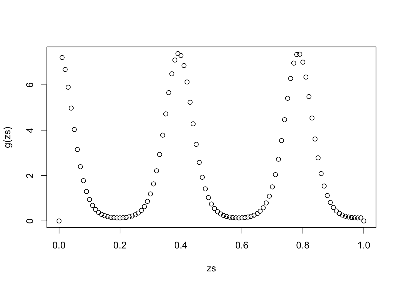

integrate(g,0,1)

2.24052 with absolute error < 2.9e-06

# Monte Carlo approximation
N <- 1000
xs <- runif(N)
mean(g(xs))

[1] 2.235894

4.1 Stratified Monte Carlo Integration

One tweak on basic Monte-Carlo is to divide \({\mathsf X}\) into \(N\) sub-regions, \({\mathsf X}_i\), and to estimate the integral within each \({\mathsf X}_i\) using a Monte Carlo approximation. This can reduce the variance of the approximation.

The underlying idea of trying to obtain the nice properties of uniform random variables, but with more even spacing over the domain of integration, is pushed to the limit by Quasi Monte Carlo integration, which uses deterministic space filling sequences of numbers as the basis for integration.

4.2 Importance sampling

In the description of Monte Carlo so far, the choice of the PDF \(\pi\) and the function \(f\) was somewhat arbitrary, up to the constraint that we require \[\pi \cdot f = g.\]

In importance sampling we make use of this flexibility (again) to write \[\int f(x) \pi(x) {\rm d}x = \int f(x) w(x) \mu(x) {\rm d}x,\] where \(w=\pi/\mu\) pointwise and again we require \(\mu(x) > 0\) whenever \(\pi(x) > 0\). This perspective is particularly helpful conceptually when we think about integrals that are already specified in terms of \(\pi\) and \(f\), such as a posterior expectation. The key message is that even if we cannot produce realizations of \(X \sim \pi\) on a computer, perhaps we can produce realizations of \(X \sim \mu\) instead and then just calculate a different Monte Carlo approximation.

Here is the previous example but where we use standard normal random variables instead of uniform random variables, just to make the point:

N <- 10000
xs <- rnorm(N)
mean(g(xs)/dnorm(xs))

[1] 2.297431

A natural question is what is the best \(\mu\) for a given integral. It turns out that this is \[\mu(x) \propto \pi(x) |f(x)|,\] which really amounts to \[\mu(x) \propto |g(x)|,\] in the original problem.

This hints at the origin of the terminology. The distribution \(\mu\) is known as the importance distribution, because at least when chosen optimally it has high density in “important” parts of the space.

4.3 Self-normalized importance sampling

One issue with importance sampling that arises often in practice is that the density \(\pi\) is only known up to a normalizing constant. More precisely, we are supposed to compute \(w(x) = \pi(x)/\mu(x)\) but we may only have access to \(\tilde{w}(x) \propto \pi(x)/\mu(x)\).

For example, \(\pi\) may be the posterior density in a simple Bayesian model with data \(y\), where the prior density and likelihood function can be computed but the normalizing constant of the posterior density is not tractable:

\[\pi(\theta) = \frac{1}{Z} \pi_0(\theta) L(\theta ; y),\] where \(Z = \int \pi_0(\theta) L(\theta ; y) {\rm d}\theta\) is the normalizing constant, also known as the marginal likelihood in this specific setting.

To compute \(\mathbb{E}_\pi (\theta)\), i.e. the posterior mean, is to compute \[\int \theta \pi(\theta) {\rm d}\theta = \frac{1}{Z} \int \theta \pi_0(\theta) L(\theta ; y) {\rm d}\theta.\] One option is to approximate the integrals \(Z\) and \(\int \theta \pi_0(\theta) L(\theta ; y) {\rm d}\theta\) separately. In fact, doing this using only one set of samples leads to what we call self-normalized importance sampling.

For simplicity, we will assume that we have realizations \(\theta_1,\ldots,\theta_N\) of i.i.d. random variables distributed according to \(\pi_0\). The importance weights are \(\tilde{w}(\theta_i) = L(\theta_i) \propto \pi(\theta)/\pi_0(\theta)\) Then the Monte Carlo approximation of the numerator is \[\frac{1}{N}\sum_{i=1}^N \theta_i L(\theta_i; y) = \frac{1}{N}\sum_{i=1}^N \theta_i \tilde{w}(\theta_i),\] while the Monte Carlo approximation of the denominator is \[\frac{1}{N}\sum_{i=1}^N L(\theta_i; y) = \frac{1}{N}\sum_{i=1}^N \tilde{w}(\theta_i),\] Now notice that if we divide the numerator by the denominator, our approximation of the posterior mean is \[\frac{\frac{1}{N}\sum_{i=1}^N \theta_i \tilde{w}(\theta_i)}{\frac{1}{N}\sum_{i=1}^N \tilde{w}(\theta_i)} = \frac{\sum_{i=1}^N \tilde{w}(\theta_i) \theta_i}{\sum_{i=1}^N \tilde{w}(\theta_i)}.\] One notices that the final expression is invariant to scaling of \(\tilde{w}\) by any constant.

The general version of the estimator is \[\tilde{I}_N = \frac{\sum_{i=1}^N \tilde{w}(X_i) f(X_i)}{\sum_{i=1}^N \tilde{w}(X_i)},\] Convergence in probability follows, e.g., by the joint convergence in probability of the numerator and denominator (each divided by \(N\)) and the continuous mapping theorem. The approximation is not unbiased in general, in contrast to importance sampling.

The sequence of approximations are asymptotically normal: \[\sqrt{N}(\tilde{I}_N-I) \to_d N(0,\sigma^2(f)),\] where \[\sigma^2(f) = \int (f(x)-I)^2 w(x) \pi(x) {\rm d} x,\] which can be smaller than the asymptotic variance of standard importance sampling, which is \(\int f(x)^2 w(x) \pi(x) {\rm d}x - I^2\).

4.4 Effective sample size

One issue with self-normalized importance sampling is that we have \(N\), say, weighted samples and these weights may vary greatly. To be precise, let us write \[\tilde{I}_N = \sum_{i=1}^N \bar{W}_i f(X_i),\] where \[\bar{W}_{i}=\frac{\tilde{w}(X_{i})}{\sum_{i=1}^{N}\tilde{w}(X_{i})}.\] The weights \(\bar{W}_i\) take values between \(0\) and \(1\), and one may be concerned that most of the weight is concentrated on a single \(\bar{W}_k\), indicating that the estimator is then almost equal to \(f(X_k)\). If \(\pi\) is not concentrated on \(X_k\) then this is problematic. The issue, of course, is that the variability of the weights alone may be compromising the quality of the estimator.

One simple measure of sample quality is the so-called “effective sample size” (ESS). It was inspired originally by quantifying the ratio of asymptotic variances with \(\mu\) and with \(\pi\): \[\frac{\int (f(x)-I)^2 w(x)^2 \mu(x) {\rm d}x}{\int (f(x)-I)^2 \pi(x) {\rm d}x},\] but this is not actually what is approximates consistently. Indeed, the ESS is a random variable that is intentionally independent of the function \(f\). The ESS is the \([1,N]\)-valued random variable \[\mathcal{E}_{N}=N\cdot\frac{\left\{ \frac{1}{N}\sum_{i=1}^{N}\tilde{w}(X_{i})\right\} ^{2}}{\left\{ \frac{1}{N}\sum_{i=1}^{N}\tilde{w}(X_{i})^{2}\right\} },\] where the fraction on the right tends to \[R(\pi,\mu)=\left\{ \int w(x)^{2}\mu(x){\rm d}x\right\} ^{-1}\in(0,1].\] One interpretation of the ESS come from the bound: \[\begin{align*} \sigma^{2}(f) &=\int(f(x)-I)^{2}w(x)^{2}\mu(x){\rm d}x \\ &\leq \left\Vert f\right\Vert _{{\rm osc}}^{2}\int w(x)^{2}\mu(x){\rm d}x \\ &=\frac{\left\Vert f\right\Vert _{{\rm osc}}^{2}}{R(\pi,\mu)}, \end{align*}\] and the effective sample size is an approximation of the denominator.

There is also a relationship to the \(\chi^{2}\)-divergence between \(\pi\) and \(\mu\): \[R(\pi,\mu)=\frac{1}{1+d_{\chi^{2}}(\pi,\mu)},\] where \[d_{\chi^2}(\pi,\mu) = \int (w(x)-1)^2 \mu(x) {\rm d}x.\]

4.5 Laplace importance sampling

One particular way to choose \(\mu\) in some settings is to use the normal approximation suggested earlier. Rather than a deterministic approximation with an error that is hard to quantify, here the idea is to use the approximation only to define a suitable importance distribution.

Let us be clear about the setting. We imagine that we are interested in the integral \[I = \int_{\mathbb{R}^d} f(x) \pi(x) {\rm d}x.\] If \(\pi\) is close to a multivariate normal distribution then it is natural to consider the approximation for the mean \(m\) and covariance matrix \(\Sigma\):

• \(m\) should be a maximizer of \(\log \pi\).
• \(\Sigma\) should be the inverse of the Hessian matrix of \(\log \pi\), \(H\), evaluated at \(m\).

We then take \(\mu = N(m,\Sigma)\) and apply importance sampling or self-normalized importance sampling.

In practice, it is sometimes a good idea to make the tails of \(\mu\) heavier than this approximation, either by inflating the covariance matrix or by using a multivariate \(t\)-distribution.

5 The log–sum–exp trick

When using self-normalized importance sampling, it is not uncommon for the weights to be on a very different scale to, say, the number \(1\). This causes numerical issues on a computer, since computers typically use inexact representations of numbers in their computations.

Consider computing the quantity \[b = \sum_{i=1}^n a_i,\] where all of the \(a_1,\ldots,a_n\) are non-negative

If all of the terms \(a_i\) are around \(\exp(-200)\) or around \(\exp(200)\) then this generally cause problems. Often we actually want to compute \(\log(b)\) if \(b\) can have a very different scale to \(1\) and similarly we should store the \(\log(a_i)\) on our computers if we want to handle very large or small quantities.

The trick is then to write \[\log(b) = \log \left ( \sum_{i=1}^n \exp(c_i) \right ),\] where \(c_i = \log(a_i)\). This is called log-sum-exp for obvious reasons. The trick is then to observe that \[\log \left ( \sum_{i=1}^n \exp(c_i) \right ) = m + \log \left ( \sum_{i=1}^n \exp(c_i - m) \right ),\] for any \(m \in \mathbb{R}\) and a suitable choice here is \[m = \max\{c_1,\ldots,c_n\}.\] The main thing to notice is that when summing \(\exp(c_i-m)\), the maximum number involved is \(\exp(0) = 1\) and if a number is so small that an underflow occurs then often this is negligible for the actual result.

6 An example

Consider a Generalised Linear Mixed Model: \[ y_i|{\bf b} \sim {\rm Poi}(\mu_i), ~~~ \log(\mu_i) = {\bf X}_i \boldsymbol{\beta}+ {\bf Z}_i {\bf b},~~~ {\bf b} \sim N({\bf 0}, \boldsymbol{\Lambda}^{-1}) \] where \(\boldsymbol{\Lambda}\) is diagonal and depends on a small number of parameters. Here, \(\boldsymbol{\beta}\) are the fixed effects and \({\bf b}\) are the random effects, with covariate matrices \({\bf X}\) and \({\bf Z}\), respectively. From the model specification it is straightforward to write down the joint probability function of \(\bf y\) and \(\bf b\), based on the factorisation \(f({\bf y}, {\bf b}) = f_{y|b}({\bf y}|{\bf b})f_b({\bf b})\). i.e. \[\begin{align*} \log\{f({\bf y}, {\bf b})\} &= \sum_i \{ y_i ({\bf X}_i \boldsymbol{\beta}+ {\bf Z}_i {\bf b}) - \exp ({\bf X}_i \boldsymbol{\beta}+ {\bf Z}_i {\bf b}) - \log(y_i!) \} - \\ & \qquad \frac{1}{2} \sum_j \lambda_j b^2_j + \frac{1}{2} \sum_j \log(\lambda_j) - \frac{1}{2} \sum_j \log(2\pi) \end{align*}\] but likelihood based inference actually requires that we can evaluate the marginal p.f. \(f_y({\bf y})\) for any values of the model parameters. Now \[ f_y({\bf y}) = \int f({\bf y}, {\bf b}) d{\bf b} \] and evaluation of this requires numerical integration.

To tie things down further, suppose that the fixed effects part of the model is simply \(\beta_0 + \beta_1 x\) where \(x\) is a continuous covariate, while the random effects part is given by two factor variables, \(z_1\) and \(z_2\), each with two levels. So a typical row of \({\bf Z}\) is a vector of 4 zeros and ones, in some order. Suppose further that the first two elements of \(\bf b\) relate to \(z_1\) and the remainder to \(z_2\) and that \({\rm diag}(\boldsymbol{\Lambda}) = [\sigma^{-2}_1,\sigma^{-2}_1,\sigma^{-2}_2,\sigma^{-2}_2]\). The following simulates 50 observations from such a model.

set.seed(1);n <- 50
x <- runif(n)
z1 <- sample(c(0,1),n,replace=TRUE)
z2 <- sample(c(0,1),n,replace=TRUE)
b <- rnorm(4) ## simulated random effects
X <- model.matrix(~x)
Z <- cbind(z1,1-z1,z2,1-z2)
eta <- X%*%c(0,3) + Z%*%b
mu <- exp(eta)
y <- rpois(n, mu)

Here is a function evaluating \(\log \{ f({\bf y},{\bf b}) \}\) (log is used here to avoid undesirable underflow to zero)

lf.yb0 <- function(y, b, theta, X, Z, lambda) {
  beta <- theta[1:ncol(X)]
  theta <- theta[-(1:ncol(X))]
  eta <- X%*%beta + Z%*%b
  mu <- exp(eta)
  lam <- lambda(theta, ncol(Z))
  sum(y*eta - mu - lfactorial(y)) - sum(lam*b^2)/2 +
      sum(log(lam))/2 - ncol(Z)*log(2*pi)/2
}

theta contains the fixed effect parameters, i.e. \(\boldsymbol{\beta}\) and the parameters of \(\boldsymbol{\Lambda}\). So in this example, theta is of length 4, with the first 2 elements corresponding to \(\boldsymbol{\beta}\) and the last two are \(\sigma_1^{-2}, \sigma_{2}^{-2}\). lambda is the name of a function for turning the parameters of \(\boldsymbol{\Lambda}\) into its leading diagonal elements, for example

var.func <- function(theta, nb) c(theta[1], theta[1], theta[2], theta[2])

Actually, for integration purposes, lf.yb0 can usefully be re-written to accept a matrix b where each column is a different \(\bf b\) at which to evaluate the log p.d.f. Suppose lf.yb is such a function. Lets try evaluating \(f_y({\bf y})\) at the simulated data, and the theta vector used for simulation, using the various integration methods covered above.

6.1 Quadrature rules

We use the Cubature package. We have the slight problem of the integration domain being infinite, but since the integrand will vanish at some distance from \({\bf b} = {\bf 0}\), we can probably safely restrict attention to the domain \([-5,5]^4\).

library(cubature)
theta <- c(0,3,1,1)
guess <- -116
my.f <- function(x) {
  exp(lf.yb0(y,x,theta,X,Z,var.func)-guess)
}
# my.integrate(my.f, rep(-5,4), rep(5,4), 10)
out <- cubintegrate(my.f,rep(-5,4), rep(5,4))
out

$integral
[1] 1.009076

$error
[1] 0.0001001912

$neval
[1] 1000065

$returnCode
[1] 0

estimated.log.density <- log(out$integral) + guess
estimated.log.density

[1] -115.991

We get an estimate, which for numerical reasons required us to have a good guess of the log of the integral. The number of function evaluations is really large at about 1 million.

6.2 Laplace approximation

To use the Laplace approximation we need to supplement lf.yb with functions glf.yb and hlf.yb which evaluate the gradient vector and Hessian of the \(\log(f)\) w.r.t. \(\bf b\). Given these functions we first find \(\hat {\bf b}\) by Newton’s method

b <- rep(0,4)
while(TRUE) {
  b0 <- b
  g <- glf.yb(y, b, theta, X, Z, var.func)
  H <- hlf.yb(y, b, theta, X, Z, var.func)
  b <- b - solve(H, g)
  b <- as.vector(b)
  if (sum(abs(b-b0)) < 1e-5*sum(abs(b)) + 1e-4) break
}
b.max <- b

after which b.max contains \(\hat {\bf b}\) and H the negative of the required \(\bf H\). It remains to evaluate the approximation

lf.yb0(y,b.max,theta,X,Z,var.func) + 2*log(2*pi) -
    0.5*determinant(H,logarithm=TRUE)$modulus

[1] -112.9528
attr(,"logarithm")
[1] TRUE

This is reasonably close to the truth, but the method itself provides us with no way of knowing how close.

6.3 Monte Carlo

Simple brute force Monte Carlo Integration follows

  N <- 100000
  lws <- rep(0,N)
  for (i in 1:N) {
    b <- -5 + 10*runif(4) # generate U([-5,5]^4) realization
    lws[i] <- lf.yb0(y, b, theta, X, Z, var.func)
  }
  log(sum(exp(lws-max(lws)))) + max(lws) - log(N) + 4*log(10)

[1] -113.7247

The next replicate gave -119.3, and the standard deviation over 100 replicates is about 2. That degree of variability is with \(10^5\) function evaluations.

6.4 Slightly better Monte Carlo

The required marginal likelihood can obviously be written \[ f_y({\bf y}) = \int f({\bf y}, {\bf b}) d{\bf b} = \int f_{y|b}({\bf y}|{\bf b})f_b({\bf b}) d{\bf b} = \mathbb{E}_b\left[f_{y|b}({\bf y}|{\bf b})\right] \] – the expectation of \(f_{y|b}\) wrt the random effects distribution. Draws from the latter must be better placed than the uniform draws used above, so this should give us a somewhat improved Monte Carlo estimator.

lf.ygb <- function(y, b, theta, X, Z, lambda) {
  beta = theta[1:ncol(X)]
  eta = Z%*%b + as.vector(X%*%beta)
  colSums(y*eta - exp(eta) - lfactorial(y))
}

N = 100000
lam = var.func(theta[3:4])
lws <- rep(0,N)
for (i in 1:N) {
  b <- rnorm(4,0,sd=sqrt(lam))
  lws[i] <- lf.ygb(y,b,theta,X,Z,var.func)
}
max(lws) + log(mean(exp(lws - max(lws))))

[1] -115.2339

The standard deviation of this scheme over 100 replicates is about 0.15. This is a modest improvement, but most of the bm samples are still wasted on regions where the integrand is negligible: exactly the situation that importance sampling addresses.

6.5 Laplace Importance Sampling

Using Laplace importance sampling allows the construction of an efficient unbiased estimate of the marginal likelihood.

N <- 10000
R <- chol(-H)
z <- matrix(rnorm(N*4),4,N)
bm <- b.max + backsolve(R,z)
lf <- lf.yb(y,bm,theta,X,Z,var.func)
zz.2 <- colSums(z*z)/2
lfz <- lf + zz.2
log(sum(exp(lfz - max(lfz)))) + max(lfz) + 2 * log(2*pi) -
    sum(log(diag(R))) - log(N)

[1] -115.2595

N <- 10000
R <- chol(-H)
lws <- rep(0,N)
for (i in 1:N) {
  z <- rnorm(4)
  b <- b.max + backsolve(R,z)
  lws[i] <- lf.yb0(y,b,theta,X,Z,var.func) + 0.5*sum(z*z)
}

log(sum(exp(lws - max(lws)))) + max(lws) + 2 * log(2*pi) -
    sum(log(diag(R))) - log(N)

[1] -115.1839

Over 100 replicates this method has a standard deviation of just under 0.001, and that is with 10 times fewer samples than the previous Monte-Carlo attempts. It drops to 0.0003 if 100000 samples are used. Stratification can reduce this variability still further. Be aware that while we know that the estimator is unbiased, it will not be on the log scale, of course.

6.6 Conclusions

The example emphasises that integration is computationally expensive, and that multi-dimensional integration is best approached by approximating the integrand with something analytically integrable or by constructing unbiased estimators of the integral. The insight that variance is likely to be minimised by concentrating the ‘design points’ of the estimator on where the integrand has substantial magnitude is strongly supported by this example, and leads rather naturally, beyond the scope of this course, to MCMC methods. Note that in likelihood maximisation settings you might also consider avoiding intractable integration via the EM algorithm (see e.g. Lange, 2010 or Monahan, 2001).