Quadrature
Error analysis is the tithe that intelligence demands of action, but it is rarely paid.
– Davis & Rabinowitz, Methods of Numerical Integration (1975), p. 208.
“Quadrature rules” are basically integral approximations using a finite number of function evaluations. All of the quadrature rules we will consider involve approximating a function using interpolating polynomials.
To focus on the main ideas, we will restrict our attention to numerically approximating the definite integral of a function \(f\) over a finite interval \([a,b]\). Extensions to semi-infinite and infinite intervals will be discussed briefly, as will extensions to multiple integrals.
In practice, for one dimensional integrals you can use R’s integrate function. For multiple integrals, the cubature package can be used. Unlike the basics covered here, these functions will produce error estimates and should be more robust.
Polynomial interpolation
We consider approximation of a continuous function \(f\) on \([a,b]\), i.e. \(f \in C^0([a,b])\) using a polynomial function \(p\). One practical motivation is that polynomials can be integrated exactly. A theoretical, high-level motivation is the Weierstrass Approximation Theorem.
Weierstrass Approximation Theorem. Let \(f \in C^0([a,b])\). There exists a sequence of polynomials \((p_n)\) that converges uniformly to \(f\) on \([a,b]\). That is, \[\Vert f - p_n \Vert_\infty = \max_{x \in [a,b]} | f(x) - p_n(x) | \to 0.\]
This suggests that for any given tolerance, there exists a polynomial that can be used to approximate a given \(C^0([a,b])\) function \(f\). However it does not indicate exactly how to construct such polynomials or, more importantly, how to do so in a computationally efficient manner without much knowledge of \(f\). Bernstein polynomials are used in a constructive proof of the theorem, but are not widely used to define polynomial approximations.
Lagrange polynomials
One way to devise an approximation is to first consider approximating \(f\) using an interpolating polynomial with, say, \(k\) points \(\{(x_i,f(x_i))\}_{i=1}^k\). The interpolating polynomial is unique, has degree at most \(k-1\), and it is convenient to express it as a Lagrange polynomial:
\[p_{k-1}(x) := \sum_{i=1}^k \ell_i(x) f(x_i),\]
where the Lagrange basis polynomials are
\[\ell_i(x) = \prod_{j=1,j\neq i}^k \frac{x-x_j}{x_i-x_j} \qquad i \in \{1,\ldots,k\}.\]
For a given 3rd degree polynomial \(f\), we plot polynomial approximations for \(k \in \{2,3,4\}\) and specific choices of \(x_1,\ldots,x_4\).
construct.interpolating.polynomial <- function(f, xs) {
  k <- length(xs)
  fxs <- f(xs)
  p <- function(x) {
    value <- 0
    for (i in 1:k) {
      fi <- fxs[i]
      zs <- xs[setdiff(1:k,i)]
      li <- prod((x-zs)/(xs[i]-zs))
      value <- value + fi*li
    }
    return(value)
  }
  return(p)
}

plot.polynomial.approximation <- function(f, xs, a, b) {
  p <- construct.interpolating.polynomial(f, xs)
  vs <- seq(a, b, length.out=500)
  plot(vs, f(vs), type='l', xlab="x", ylab="black: f(x), red: p(x)")
  points(xs, f(xs), pch=20)
  lines(vs, vapply(vs, p, 0), col="red")
}

a <- -4
b <- 4

f <- function(x) {
  return(-x^3 + 3*x^2 - 4*x + 1)
}

plot.polynomial.approximation(f, c(-2, 2), a, b)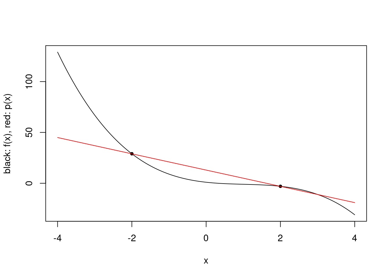
plot.polynomial.approximation(f, c(-2, 0, 2), a, b)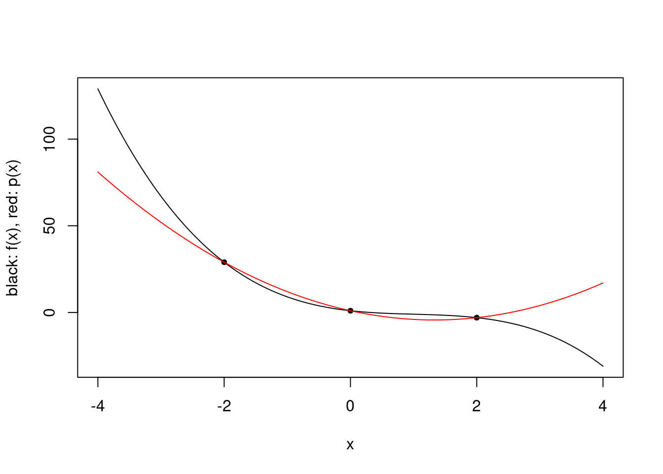
plot.polynomial.approximation(f, c(-2, 0, 2, 4), a, b)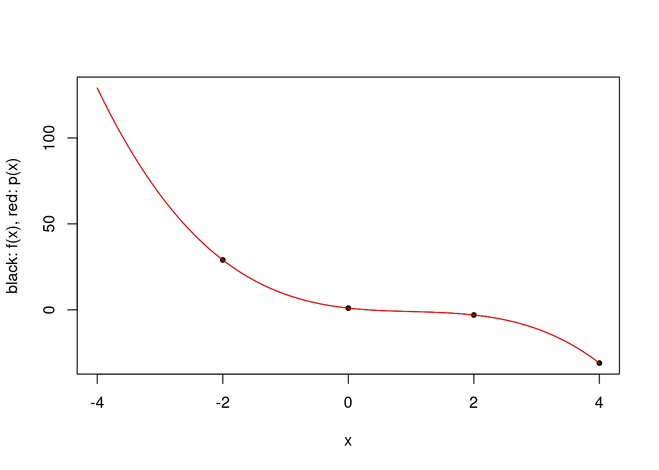
Of course, one might instead want a different representation of the polynomial, e.g. as sums of monomials with appropriate coefficients.
\[p(x) = \sum_{i=1}^k a_i x^{i-1}.\]
This can be accomplished in principle by solving a linear system. In practice, this representation is often avoided for large \(k\) as solving the linear system is numerically unstable.
construct.vandermonde.matrix <- function(xs) {
  k <- length(xs)
  A <- matrix(0, k, k)
  for (i in 1:k) {
    A[i,] <- xs[i]^(0:(k-1))
  }
  return(A)
}

compute.monomial.coefficients <- function(f, xs) {
  fxs <- f(xs)
  A <- construct.vandermonde.matrix(xs)
  coefficients <- solve(A, fxs)
  return(coefficients)
}

construct.polynomial <- function(coefficients) {
  k <- length(coefficients)
  p <- function(x) {
    return(sum(coefficients*x^(0:(k-1))))
  }
  return(p)
}

xs <- c(-2,0,2)
p <- construct.polynomial(compute.monomial.coefficients(f, xs))
plot.polynomial.approximation(f, xs, a, b)
vs <- seq(-4, 4, length.out=100)
lines(vs, vapply(vs, p, 0), col="blue", lty="dashed")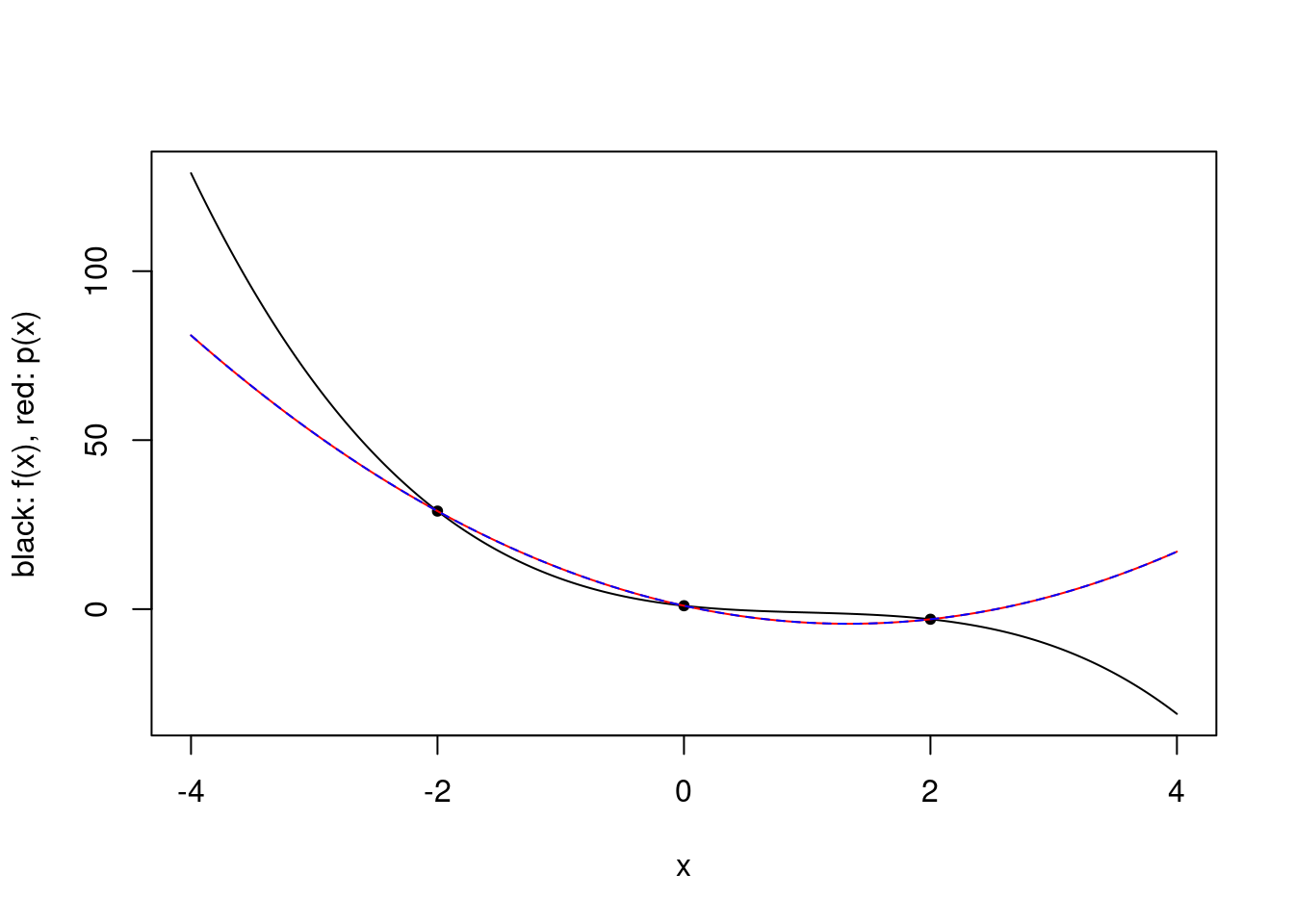
Polynomial interpolation error
It is clear that by choosing \(k\) large enough, one can approximate any polynomial. On the other hand, one is typically interested in approximating functions that are not polynomials.
Interpolation Error Theorem. Let \(f \in C^{k}[a,b]\), i.e. \(f : [a,b] \to \mathbb{R}\) has \(k\) continuous derivatives, and \(p_{k-1}\) be the polynomial interpolating \(f\) at the \(k\) points \(x_1,\ldots,x_k\). Then for any \(x \in [a,b]\) there exists \(\xi \in (a,b)\) such that \[\begin{equation} \tag{1} f(x)-p_{k-1}(x) = \frac{1}{k!} f^{(k)}(\xi) \prod_{i=1}^k (x-x_i). \end{equation}\]
The Interpolation Error Theorem is encouraging, but it does not provide immediately any guarantee that an obvious sequence of interpolating polynomials will converge uniformly or even pointwise to \(f\). In fact, there is a sequence of interpolation points that guarantees uniform convergence.
Theorem. Let \(f \in C^{0}[a,b]\). There exists a sequence of sets of interpolation points \(X_1, X_2, \ldots\) such that the corresponding sequence of interpolating polynomials converges uniformly to \(f\) on \([a,b]\).
This theorem does not quite follow from the Weierstrass Approximation Theorem, since that theorem made no mention that the polynomials can be interpolating polynomials. One might wonder if it is possible to define a universal sequence of sets of interpolating points \(X_1,X_2,\ldots\) that does not depend on the function \(f\) while retaining (uniform) convergence. Unfortunately this is not possible: for any fixed sequence of sets of interpolation points there exists a continuous function \(f\) for which the sequence of interpolating polynomials diverges.
An example of a fixed sequence of sets of interpolation points is to let \(X_k\) be the set of \(k\) uniformly spaced points including \(a\), and \(b\) if \(k>1\). This sequence of sets may work well for many functions, such as \(\log\) on \([1,2]\).
construct.uniform.point.set <- function(a, b, k) {
  if (k==1) return(a)
  return(seq(a, b, length.out=k))
}

a <- 1
b <- 2
plot.polynomial.approximation(log, construct.uniform.point.set(a, b, 10), a, b)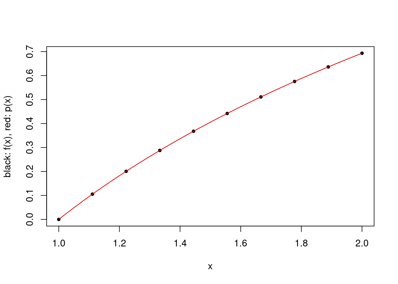
However, there are functions for which uniformly spaced points are not suitable. A famous example is the Runge function \(x \mapsto 1/(1+25x^2)\) on \([-1,1]\). For \(k=50\), the polynomial approximation is very poor close to the ends of the interval, and the situation does not improve by increasing \(k\).
a <- -1
b <- 1
f <- function(x) return(1/(1+25*x^2))
plot.polynomial.approximation(f, construct.uniform.point.set(a,b,50), a, b)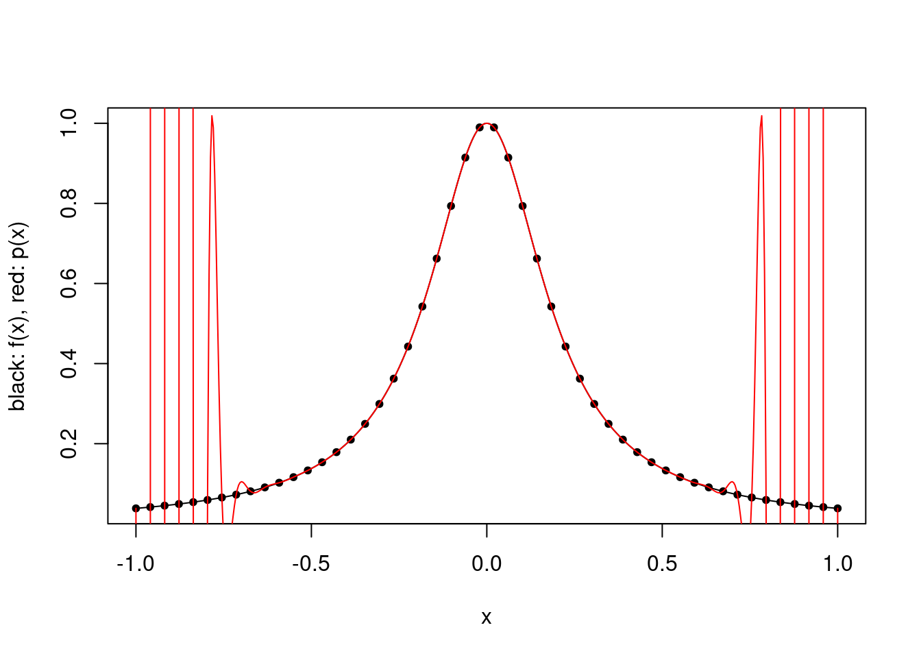
This does not contradict the Interpolation Error Theorem because the maximum over \([-1,1]\) of the \(k\)th derivative of the Runge function grows very quickly with \(k\), and in particular more quickly than the product term decreases with \(k\).
Another example is to take the function \(x \mapsto |x|\) on \([-1,1]\).
a <- -1
b <- 1
plot.polynomial.approximation(abs, construct.uniform.point.set(a,b,50), a, b)
This does not contradict the Interpolation Error Theorem because \(x \mapsto |x|\) is not differentiable at \(0\).
It is possible to mitigate this issue to some extent by choosing the interpolation points more carefully. For example, one can choose the points for each \(k\) so as to minimize the maximum absolute value of the product term in (1), which gives the Chebyshev points. Specifically, for a given \(k\), one chooses the points \[\cos \left (\frac{2i-1}{2k}\pi \right ),\qquad i\in \{1,\ldots,k\},\] and the absolute value of the product term is then bounded above by \(2^{1-k}\).
These points do not minimize the overall error, because \(\xi\) implicitly depends on the interpolation points as well. For the Runge and absolute value functions, these points lead to a very good approximation using 50 points.
construct.chebyshev.point.set <- function(k) {
  return(cos((2*(1:k)-1)/2/k*pi))
}

plot.polynomial.approximation(f, construct.chebyshev.point.set(50), a, b)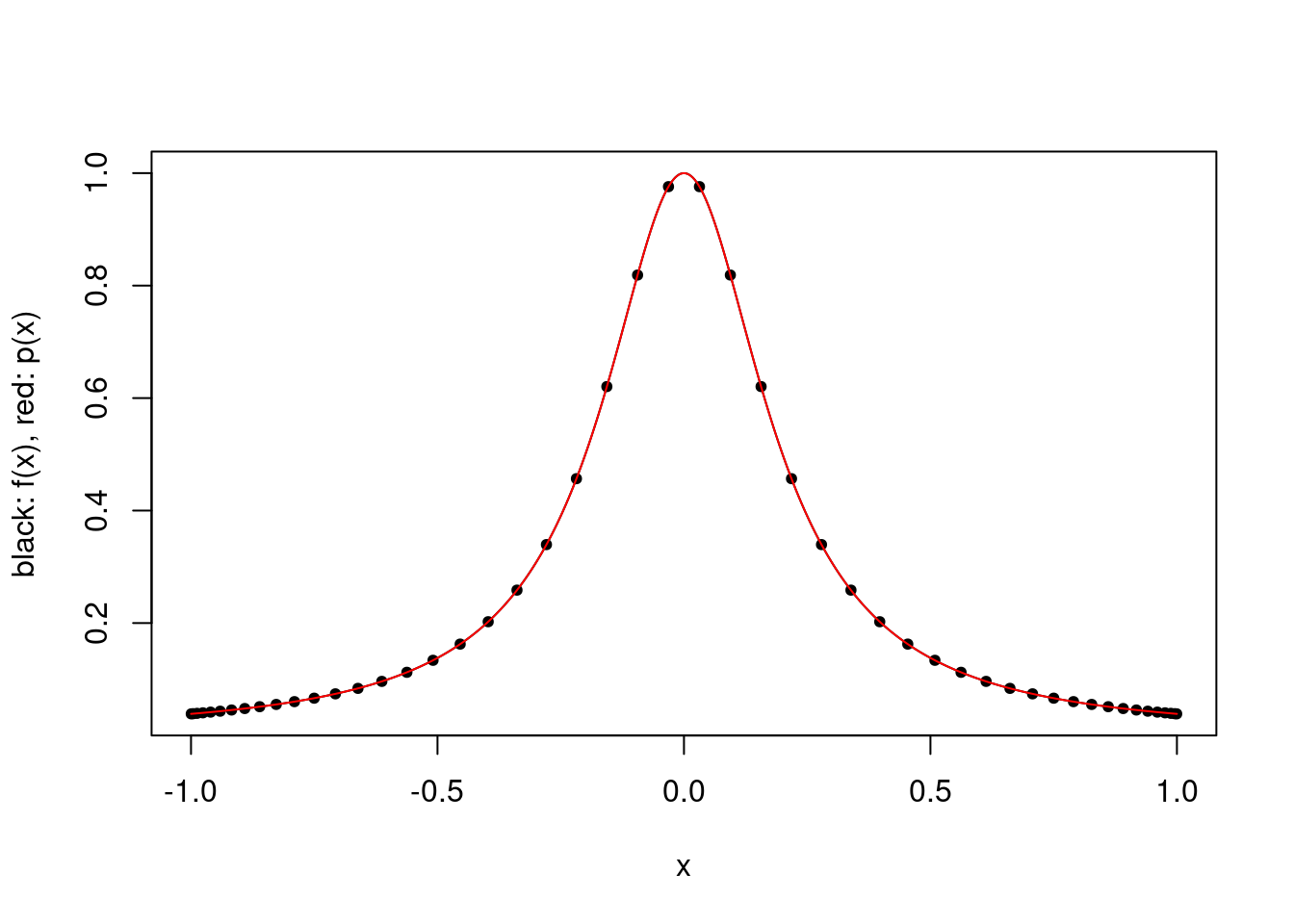
plot.polynomial.approximation(abs, construct.chebyshev.point.set(50), a, b)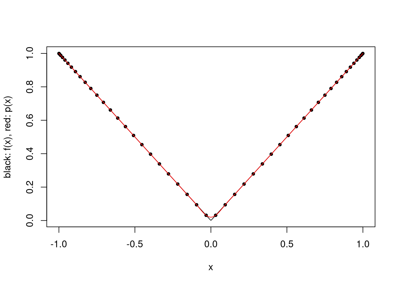
You may notice that these points are clustered around \(-1\) and \(1\).
hist(construct.chebyshev.point.set(10000))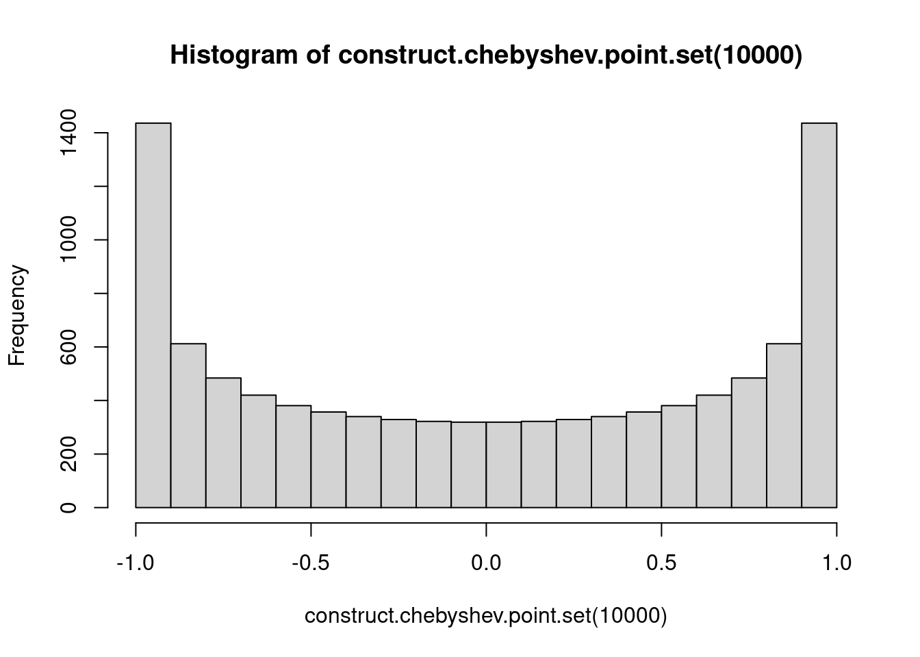
This is not a complete solution: there exist functions for which the interpolating polynomial obtained using Chebyshev points diverges, but these are usually quite complicated. Moreover, the reduction in absolute value of the product term in the error expression is not sufficient to explain the improved performance for the Runge function, and the Interpolation Error Theorem says nothing about functions that are not differentiable such as \(x \mapsto |x|\).
Composite polynomial interpolation
An alternative to using many interpolation points to fit a high-degree polynomial is to approximate the function with different polynomials in a number of subintervals of the domain. This results in a piecewise polynomial approximation that is not necessarily continuous.
We consider a simple scheme where \([a,b]\) is partitioned into a number of equal length subintervals, and within each subinterval \(k\) interpolation points are used to define an approximating polynomial. To keep things simple, we consider only two possible ways to specify the \(k\) interpolation points within each subinterval. In both cases the points are evenly spaced and evenly spaced from the endpoints of the interval. However, when the scheme is “closed”, the endpoints of the interval are included, while when the scheme is “open”, the endpoints are not included. For a closed scheme with \(k=1\), we opt to include the left endpoint.
# get the endpoints of the subintervals
get.subinterval.points <- function(a, b, nintervals) {
  return(seq(a, b, length.out=nintervals+1))
}

# returns which subinterval a point x is in
get.subinterval <- function(x, a, b, nintervals) {
  h <- (b-a)/nintervals
  return(min(max(1,ceiling((x-a)/h)),nintervals))
}

# get the k interpolation points in the interval
# this depends on the whether the scheme is open or closed
get.within.subinterval.points <- function(a, b, k, closed) {
  if (closed) {
    return(seq(a, b, length.out=k))
  } else {
    h <- (b-a)/(k+1)
    return(seq(a+h,b-h,h))
  }
}

construct.piecewise.polynomial.approximation <- function(f, a, b, nintervals, k, closed) {
  ps <- vector("list", nintervals)
  subinterval.points <- get.subinterval.points(a, b, nintervals)
  for (i in 1:nintervals) {
    left <- subinterval.points[i]
    right <- subinterval.points[i+1]
    points <- get.within.subinterval.points(left, right, k, closed)
    p <- construct.interpolating.polynomial(f, points)
    ps[[i]] <- p
  }
  p <- function(x) {
    return(ps[[get.subinterval(x, a, b, nintervals)]](x))
  }
  return(p)
}

plot.piecewise.polynomial.approximation <- function(f, a, b, nintervals, k, closed) {
  p <- construct.piecewise.polynomial.approximation(f, a, b, nintervals, k, closed)
  vs <- seq(a, b, length.out=500)
  plot(vs, f(vs), type='l', xlab="x", ylab="black: f(x), red: p(x)")
  lines(vs, vapply(vs, p, 0), col="red")
  subinterval.points <- get.subinterval.points(a, b, nintervals)
  for (i in 1:nintervals) {
    left <- subinterval.points[i]
    right <- subinterval.points[i+1]
    pts <- get.within.subinterval.points(left, right, k, closed)
    points(pts, f(pts), pch=20, col="blue")
  }
  abline(v = subinterval.points)
}
plot.piecewise.polynomial.approximation(sin, 0, 10, 5, 1, TRUE)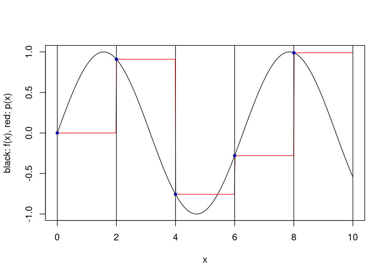
plot.piecewise.polynomial.approximation(sin, 0, 10, 5, 2, TRUE)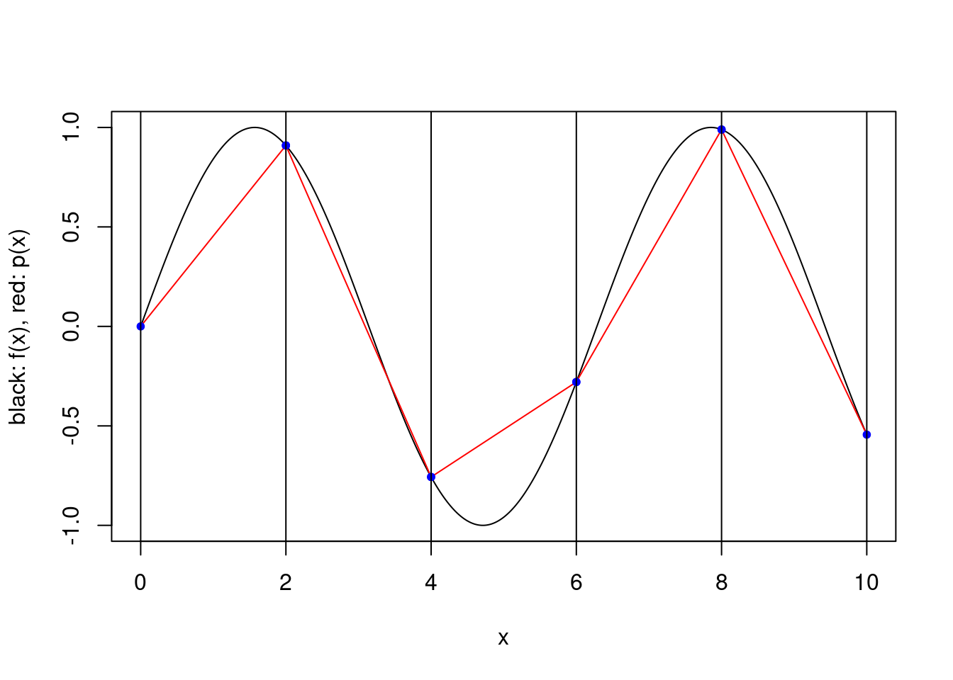
plot.piecewise.polynomial.approximation(sin, 0, 10, 5, 2, FALSE)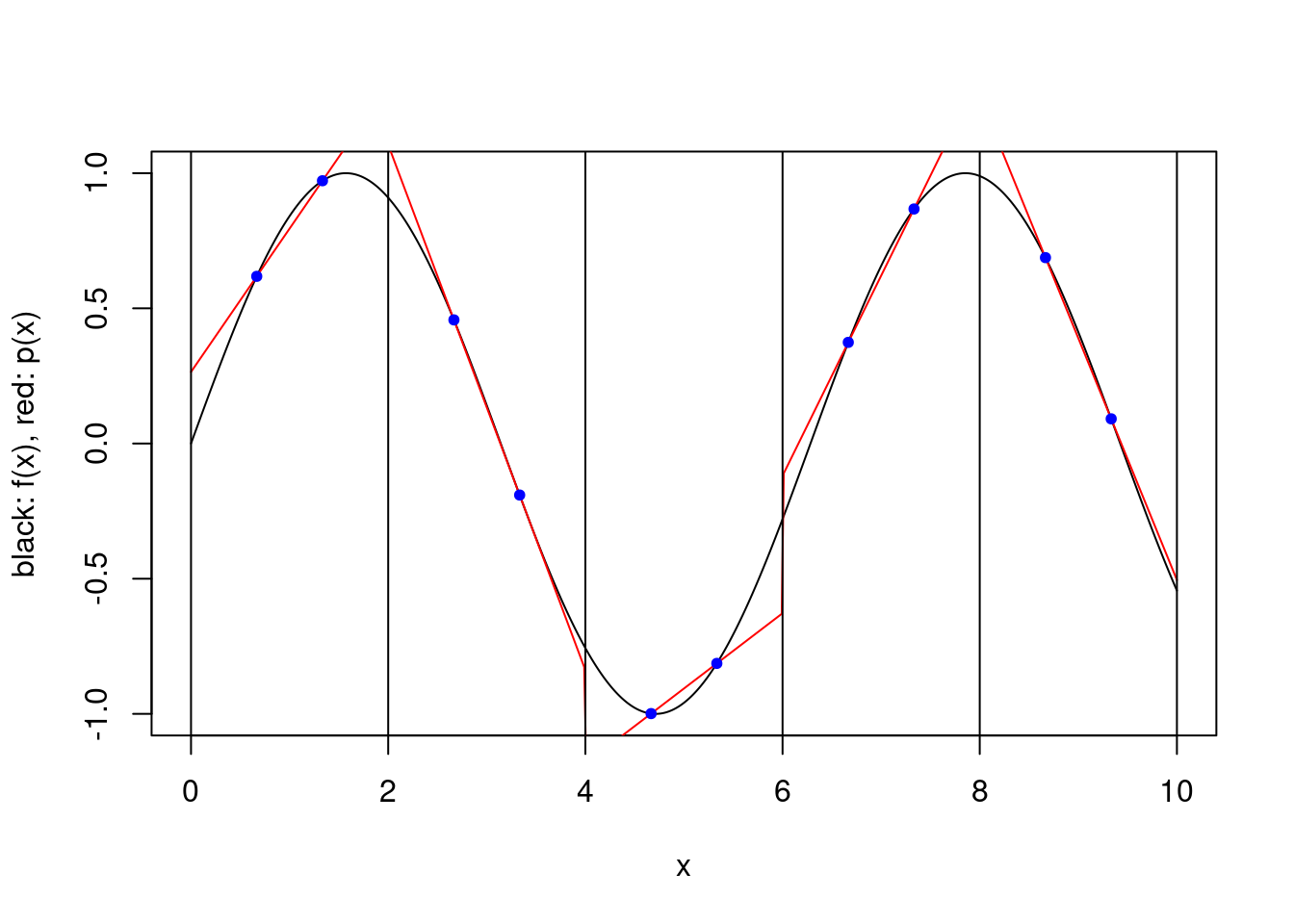
plot.piecewise.polynomial.approximation(sin, 0, 10, 5, 3, TRUE)
plot.piecewise.polynomial.approximation(sin, 0, 10, 20, 1, TRUE)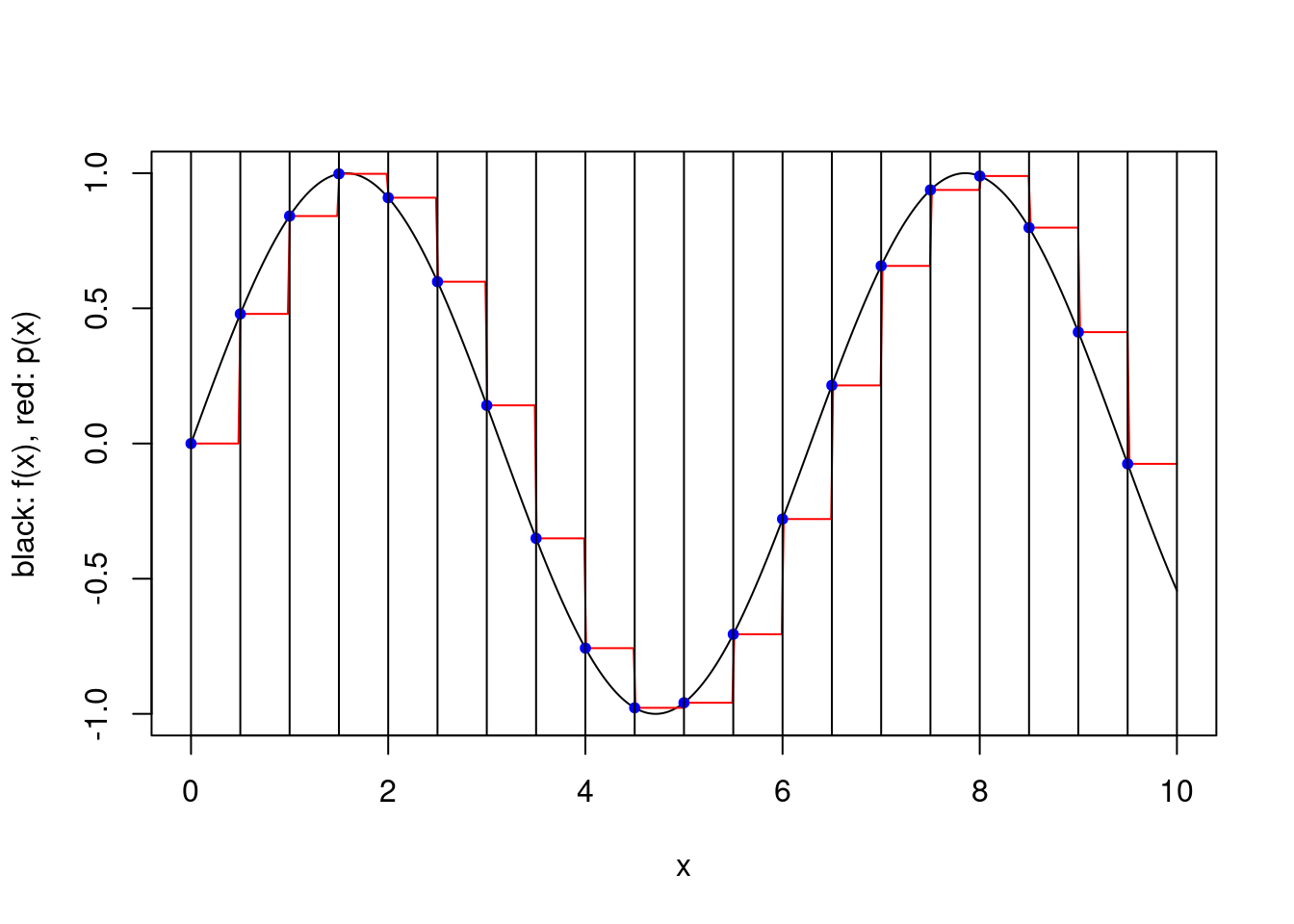
plot.piecewise.polynomial.approximation(sin, 0, 10, 20, 1, FALSE)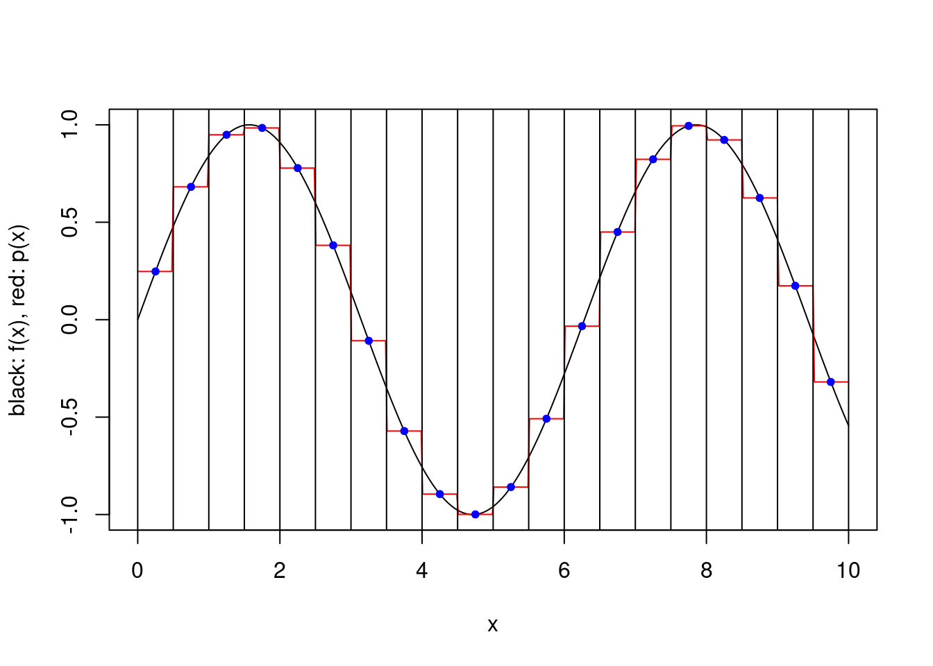
The error associated with the approximation can be obtained using the Interpolation Error Theorem. In particular, one can see that for a large number of subintervals the product term in (1) can be made arbitrarily small in absolute value. If one chooses, say, \(k=1\) (resp. \(k=2\)) and the function is almost constant (resp. linear) on small intervals, the approximation error can then be made very small.
Other polynomial interpolation schemes
There are other polynomial interpolation schemes. For example, one might fit a polynomial using derivatives of \(f\) as well as \(f\) itself, which is known as Hermite interpolation. The idea of incorporating derivatives into piecewise polynomial interpolation, e.g. by matching derivatives at the boundaries of the subintervals is known as spline interpolation. This ensures that the piecewise polynomial approximation has a certain number of continuous derivatives.
In addition, there are a number of different function approximation schemes that use more complicated approximating functions and do not necessarily involve interpolation. For example, artificial neural networks are used to approximate high-dimensional functions. However, it may not be easy to integrate complicated approximating functions.
Polynomial integration
We now consider approximating the integral
\[I(f) := \int_a^b f(x) {\rm d}x,\]
where \(f \in C^0([a,b])\).
All of the approximations we will consider here involve computing integrals associated with the polynomial approximations. The approximations themselves are often referred to as quadrature rules.
Changing the limits of integration
For constants \(a<b\) and \(c<d\), we can accommodate a change of finite interval via
\[\int_a^b f(x) {\rm d}x = \int_c^d g(y) {\rm d}y,\]
by defining
\[g(y) := \frac{b-a}{d-c} f \left (a+\frac{b-a}{d-c}(y-c) \right ).\]
Examples of common intervals are \([-1,1]\) and \([0,1]\).
change.domain <- function(f, a, b, c, d) {
  g <- function(y) {
    return((b-a)/(d-c)*f(a + (b-a)/(d-c)*(y-c)))
  }
  return(g)
}

# test out the function using R's integrate function
integrate(sin, 0, 10)
## 1.839072 with absolute error < 9.9e-12g = change.domain(sin, 0, 10, -1, 1)
integrate(g, -1, 1)## 1.839072 with absolute error < 9.9e-12One can also accommodate a semi-infinite interval by a similar change of variables. One example is
\[\int_a^\infty f(x) {\rm d}x = \int_0^1 g(y) {\rm d}y, \qquad g(y) := \frac{1}{(1-y)^2} f \left ( a + \frac{y}{1-y} \right ).\]
Similarly, one can transform an integral over \(\mathbb{R}\) to one over \([-1,1]\)
\[\int_{-\infty}^\infty f(x) {\rm d}x = \int_{-1}^1 g(t) {\rm d}t, \qquad g(t) := \frac{1+t^2}{(1-t^2)^2} f \left ( \frac{t}{1-t^2} \right ).\]
We will only consider finite intervals here.
Integrating the interpolating polynomial approximation
Consider integrating a Lagrange polynomial \(p_{k-1}\) over \([a,b]\). We have \[\begin{align} I(p_{k-1}) &= \int_a^b p_{k-1}(x) {\rm d}x \\ &= \int_a^b \sum_{i=1}^k \ell_i(x) f(x_i) {\rm d}x \\ &= \sum_{i=1}^k f(x_i) \int_a^b \ell_i(x) {\rm d}x \\ &= \sum_{i=1}^k w_i f(x_i), \end{align}\] where for \(i \in \{1,\ldots,k\}\), \(w_i := \int_a^b \ell_i(x) {\rm d}x\) and we recall that \(\ell_i(x) = \prod_{j=1,j\neq i}^k \frac{x-x_j}{x_i-x_j}\).
The approximation of \(I(f)\) is \(\hat{I}(f) = I(p_{k-1})\), where \(p_{k-1}\) depends only on the choice of interpolating points \(x_1,\ldots,x_k\).
The functions \(\ell_i\) can be a bit complicated, but certainly can be integrated by hand quite easily for small values of \(k\). For example, with \(k=1\) we have \(\ell_1 \equiv 1\), so the integral \(\int_a^b \ell_1(x) {\rm d}x = b-a\). For \(k=2\) we have \(\ell_1(x) = (x-x_2)/(x_1-x_2)\), yielding \[\int_a^b \ell_1(x) {\rm d}x = \frac{b-a}{2(x_1-x_2)}(b+a-2x_2),\] and similarly \(\ell_2(x) = (x-x_1)/(x_2-x_1)\), so \[\int_a^b \ell_2(x) {\rm d}x = \frac{b-a}{2(x_2-x_1)}(b+a-2x_1).\]
Newton–Cotes rules
The rectangular rule corresponds to a closed scheme with \(k=1\):
\[\hat{I}_{\rm rectangular}(f) = (b-a) f(a).\]
The midpoint rule corresponds to an open scheme with \(k=1\):
\[\hat{I}_{\rm midpoint}(f) = (b-a) f \left ( \frac{a+b}{2} \right).\]
The trapezoidal rule corresponds to a closed scheme with \(k=2\). Since \((x_1,x_2) = (a,b)\), we obtain \(\int_a^b \ell_1(x) {\rm d}x = (b-a)/2\) and
\[\hat{I}_{\rm trapezoidal}(f) = \frac{b-a}{2} \{ f(a)+f(b) \}.\]
Simpson’s rule corresponds to a closed scheme with \(k=3\). After some calculations, we obtain
\[\hat{I}_{\rm Simpson}(f) = \frac{b-a}{6} \left \{ f(a) + 4 f \left ( \frac{a+b}{2} \right) + f(b) \right \}.\]
We can obtain a very crude bound on the error of integration using any sequence of interpolation points.
Theorem. Let \(f \in C^k([a,b])\). Then the integration error for interpolation points \(x_1,\ldots,x_k\) satisfies \[| \hat{I}(f) - I(f) | \leq \max_{\xi \in [a,b]} |f^{(k)}(\xi)| \frac{(b-a)^{k+1}}{k!}.\]
Proof. We have, with \(\xi(x) \in (a,b)\) for each \(x\), \[\begin{align} | \hat{I}(f) - I(f) | &= \left | \int_a^b p_{k-1}(x) - f(x) {\rm d}x \right | \\ &\leq \int_a^b \left | p_{k-1}(x) - f(x) \right | {\rm d}x \\ &= \int_a^b \left | \frac{1}{k!} f^{(k)}(\xi(x)) \prod_{i=1}^k (x-x_i) \right | {\rm d}x \\ &= \frac{1}{k!} \int_a^b \left |f^{(k)}(\xi(x))\right | \prod_{i=1}^k |x-x_i| {\rm d}x \\ & \leq \max_{\xi \in [a,b]} \left |f^{(k)}(\xi)\right | \frac{(b-a)^{k+1}}{k!}. \end{align}\]
The theorem can only really be used to justify low error estimates when \(b-a\) is small or \(f\) is a polynomial of degree \(k\).
The crude nature of the bound does mean that it misses some interesting subtleties. A more refined treatment of the error can show the following.
| rule | \(\hat{I}(f) - I(f)\), with \(\xi \in (a,b)\) |
|---|---|
| rectangular | \(-\frac{1}{2}(b-a)^2 f'(\xi)\) |
| midpoint | \(-\frac{1}{24}(b-a)^3 f^{(2)}(\xi)\) |
| trapezoidal | \(\frac{1}{12}(b-a)^3 f^{(2)}(\xi)\) |
| Simpson | \(\frac{1}{2880}(b-a)^5 f^{(4)}(\xi)\) |
This indicates that the midpoint rule, which uses only one point, is often better than the trapezoidal rule, which uses 2. These are both significantly worse than Simpson’s rule, which uses 3 points. One might think that using large numbers of points is beneficial, but this is not always the case since the interpolating polynomial may become quite poor when using equally spaced points as seen before. We also see that the rectangular and trapezoidal rules are exact for constant functions, the midpoint rule is exact for linear functions, and Simpson’s rule is exact for polynomials of degree up to 3.
newton.cotes <- function(f, a, b, k, closed) {
  if (k == 1) {
    if (closed) {
      return((b-a)*f(a))
    } else {
      return((b-a)*f((a+b)/2))
    }
  }
  if (k == 2 && closed) {
    return((b-a)/2*(f(a)+f(b)))
  }
  if (k == 3 && closed) {
    return((b-a)/6*(f(a)+4*f((a+b)/2)+f(b)))
  }
  stop("not implemented")
}

nc.example <- function(f, name, value) {
  df <- data.frame(f=character(), rule=character(), error=numeric())
  df <- rbind(df, data.frame(f=name, rule="Rectangular", error=newton.cotes(f,0,1,1,TRUE)-value))
  df <- rbind(df, data.frame(f=name, rule="Midpoint", error=newton.cotes(f,0,1,1,FALSE)-value))
  df <- rbind(df, data.frame(f=name, rule="Trapezoidal", error=newton.cotes(f,0,1,2,TRUE)-value))
  df <- rbind(df, data.frame(f=name, rule="Simpson's", error=newton.cotes(f,0,1,3,TRUE)-value))
  return(df)
}

df <- nc.example(function(x) x, "x", 1/2)
df <- rbind(df, nc.example(function(x) x^2, "x^2", 1/3))
df <- rbind(df, nc.example(function(x) x^3, "x^3", 1/4))
df <- rbind(df, nc.example(function(x) x^4, "x^4", 1/5))

ggplot(df, aes(fill=rule, y=error, x=f)) + geom_bar(position="dodge", stat="identity")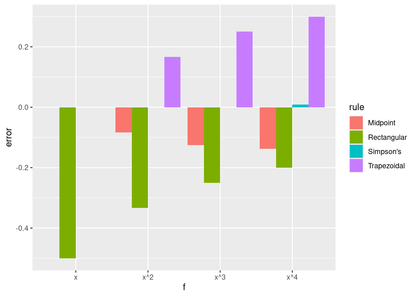
Composite rules
When a composite polynomial interpolation approximation is used, the integral of the approximation is simply the sum of the integrals associated with each subinterval. Hence, a composite Newton–Cotes rule is obtained by splitting the interval \([a,b]\) into \(m\) subintervals and summing the approximate integrals from the Newton–Cotes rule for each subinterval. \[\hat{I}^m_{\rm rule}(f) = \sum_{i=1}^m \hat{I}_{\rm rule}(f_i),\] where \(f_i\) is \(f\) restricted to \([a+(i-1)h, a+ih]\) and \(h=(b-a)/m\).
composite.rule <- function(f, a, b, subintervals, rule) {
  subinterval.points <- get.subinterval.points(a, b, subintervals)
  s <- 0
  for (i in 1:subintervals) {
    left <- subinterval.points[i]
    right <- subinterval.points[i+1]
    s <- s + rule(f, left, right)
  }
  return(s)
}

# composite Newton--Cotes
composite.nc <- function(f, a, b, subintervals, k, closed) {
  rule <- function(f, left, right) {
    newton.cotes(f, left, right, k, closed)
  }
  return(composite.rule(f, a, b, subintervals, rule))
}Proposition. Let \([a,b]\) be split into \(m\) subintervals of length \(h = (b-a)/m\). Assume that the quadrature rule used in each subinterval has error \(C h^r f^{(s)}(\xi)\) for some \(r, s \in \mathbb{N}\). Then the error for the composite rule is \[C \frac{(b-a)^r}{m^{r-1}} f^{(s)}(\xi),\] where \(\xi \in (a,b)\).
Proof. We have, with \(\xi_i\) in the \(i\)th subinterval, \[\begin{align} \hat{I}^m(f) - I(f) &= \sum_{i=1}^m \hat{I}(f_i) - I(f_i) \\ &= \sum^m_{i=1} C h^r f^{(s)}(\xi_i) \\ &= C \frac{(b-a)^r}{m^{r-1}} \frac{1}{m} \sum^m_{i=1} f^{(s)}(\xi_i) \\ &= C \frac{(b-a)^r}{m^{r-1}} f^{(s)}(\xi). \end{align}\]
We obtain the following composite errors, in which the dependence on \(m\) is of particular interest.
| rule | \(\hat{I}^m(f) - I(f)\), with \(\xi \in (a,b)\) |
|---|---|
| rectangular | \(-\frac{1}{2m}(b-a)^2 f'(\xi)\) |
| midpoint | \(-\frac{1}{24m^2}(b-a)^3 f^{(2)}(\xi)\) |
| trapezoidal | \(\frac{1}{12m^2}(b-a)^3 f^{(2)}(\xi)\) |
| Simpson | \(\frac{1}{2880m^4}(b-a)^5 f^{(4)}(\xi)\) |
We plot the errors against their theoretical values for \(f = \sin\), \((a,b) = (0,10)\) and different numbers of subintervals, \(m\). We replace \(f^{(s)}(\xi)\) in the theoretical expression with \((b-a)^{-1} \int_a^b f^{(s)}(x) {\rm d}x\), which should be accurate for large values of \(m\).
ms <- c(10:19, seq(20, 500, 10))

composite.rectangular <- vapply(ms, function(m) composite.nc(sin, 0, 10, m, 1, TRUE), 0)

composite.midpoints <- vapply(ms, function(m) composite.nc(sin, 0, 10, m, 1, FALSE), 0)

composite.trapezoidal <- vapply(ms, function(m) composite.nc(sin, 0, 10, m, 2, TRUE), 0)

composite.simpsons <- vapply(ms, function(m) composite.nc(sin, 0, 10, m, 3, TRUE), 0)

val <- 1-cos(10) # integral of sin(x) for x=0..10
v1 <- -sin(10)/10 # integral of sin'(x)/10 for x=0..10
v2 <- val/10 # integral of sin(x)/10 for x=0..10

tr <- tibble(m=ms, rule="rectangular", log.error=log(composite.rectangular - val),
             theory=log(v1*1/2*10^2/ms))
tt <- tibble(m=ms, rule="trapezoidal", log.error=log(val - composite.trapezoidal),
             theory=log(v2*1/12*10^3/ms^2))
tm <- tibble(m=ms, rule="midpoints", log.error=log(composite.midpoints - val),
            theory=log(v2*1/24*10^3/ms^2))
ts <- tibble(m=ms, rule="simpsons", log.error=log(composite.simpsons - val),
            theory=log(v2*1/2880*10^5/ms^4))
tib <- bind_rows(tr, tt, tm, ts)
ggplot(tib, aes(x=m, colour=rule)) + geom_point(aes(y=log.error)) + geom_line(aes(y=theory))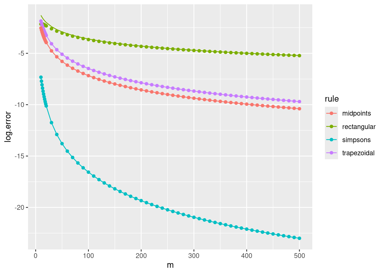
Gaussian quadrature
We have seen that when approximating a non-polynomial function by an interpolating polynomial, it can be advantageous to use Chebyshev points rather than uniformly spaced points. We pursue here a related but different approach, specific to quadrature. We again wish to exploit the freedom to choose interpolation points but instead of trying to reduce \(\Vert f - p_{k-1} \Vert_\infty\) we want to reduce the error of the approximate integral.
We consider a weighted integral \[I = \int_a^b f(x) w(x) {\rm d} x,\] where \(w\) is continuous and positive on \((a,b)\) and for every \(n \in \mathbb{N}\), \(\int_a^b x^n w(x) {\rm d}x\) is finite. For intuition, and for easy comparison with the techniques discussed so far one can consider the case \(w \equiv 1\).
Two functions \(f\) and \(g\) are orthogonal on the function space \[L^2_w([a,b]) := \left \{ f: \int_a^b f(x)^2 w(x) {\rm d}x < \infty \right \},\] if \[\langle f,g \rangle_{L^2_w([a,b])} = \int_a^b f(x)g(x)w(x) {\rm d}x = 0.\] There exists a unique sequence of orthogonal polynomials \(p_0,p_1,\ldots\) in \(L^2_w([a,b])\) that are monic, i.e. the degree of \(p_k\) is \(k\) and the leading coefficient is \(1\). These can be constructed by the Gram–Schmidt process using the initial functions \(1,x,x^2,\ldots\), renormalizing to make the polynomials monic. For example, with \((a,b) = (-1,1)\) and \(w \equiv 1\) this procedure generates the (monic) Legendre polynomials: the corresponding quadrature rule is called Gauss–Legendre quadrature.
In addition to existing and being unique up to scaling, each orthogonal polynomial of degree \(n\) has \(n\) distinct roots that lie in \((a,b)\). In fact, the \(k\) roots of \(p_k\) are the interpolation points for a Gaussian quadrature rule.
Theorem. Let \(p_k\) be the \(k\)th orthogonal polynomial in \(L^2_w([a,b])\) and \(x_1,\ldots,x_k\) its roots. Let \(\hat{I}(f) = \sum_{i=1}^k w_i f(x_i)\), where \(w_i = \int_a^b w(x) \ell_i(x) {\rm d}x\). Then if \(f\) is a degree \(2k-1\) polynomial, \(\hat{I}(f) = I(f) = \int_a^b f(x) w(x) {\rm d}x\).
Proof. We can write \(f = p_k q + r\), where \(q\) and \(r\) are both polynomials of degree less than or equal to \(k-1\). It follows that \[I(f) = \int_a^b \{ p_k(x)q(x) + r(x) \} w(x) {\rm d}x = \int_a^b r(x) w(x) {\rm d}x = I(r),\] since \(q\) is a linear combination of \(p_0,\ldots,p_{k-1}\), which are all orthogonal to \(p_k\) in \(L^2_w([a,b])\). Moreover, \[\hat{I}(f) = \sum_{i=1}^k w_i \{ p_k(x_i) q(x_i) + r(x_i) \} = \sum_{i=1}^k w_i r(x_i) = \hat{I}(r),\] since \(p_k(x_i) = 0\) for each \(i \in \{1,\ldots,k\}\). Therefore, \(\hat{I}(f) = \hat{I}(r)\) approximating \(I(f) = I(r)\) is a \(k\)-point interpolating polynomial quadrature rule where \(r\) is a polynomial of degree less than or equal to \(k-1\), and hence \(\hat{I}(f) = \hat{I}(r) = I(r) = I(f)\).
We consider a simple example with a degree 5 polynomial \(f(x) = x^5 + x^4 + x^3 + x^2 + x + 1\), \(w \equiv 1\), and we use the roots of \(p_3(x) = x^3 - 0.6x\) as the 3 interpolation points. It is straightforward to plot \(f\) and the interpolating polynomial, and clearly the approximation is not exact.
pts <- c(-sqrt(3/5), 0, sqrt(3/5))
f <- function(x) 1 + x + x^2 + x^3 + x^4 + x^5
plot.polynomial.approximation(f, pts, -1, 1)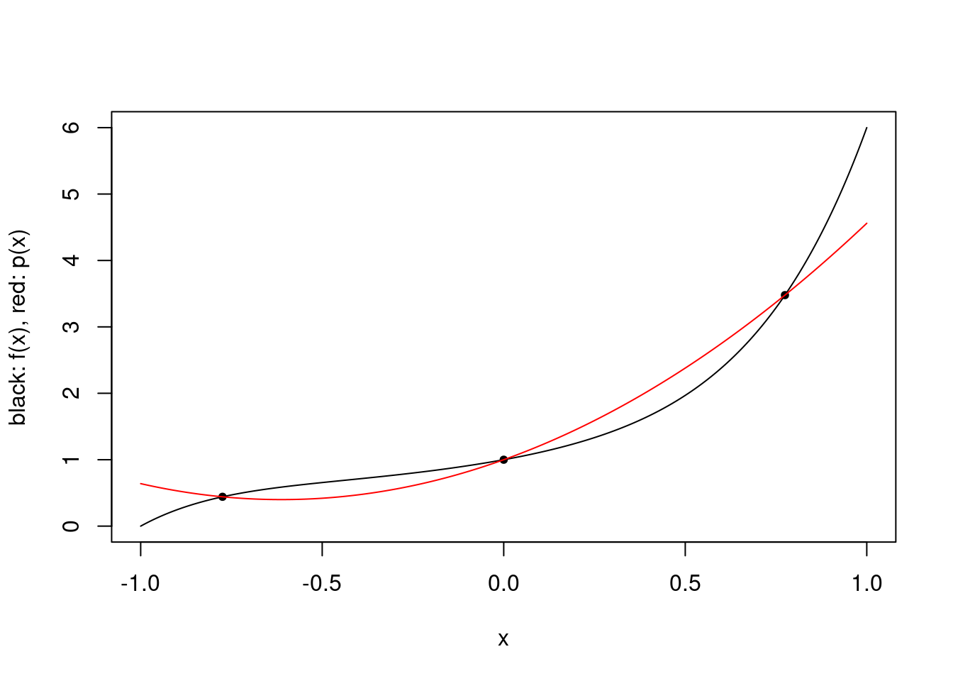
For this function, the quotient polynomial \(f/p_3\) is \(q(x) = x^2+x+1.6\) and the remainder polynomial is \(r(x) = 1.6x^2+1.96x+1\). For intuition, we can plot the polynomial approximation of \(f - r = p_3 q\).
p3 <- function(x) x^3 - 0.6*x
q <- function(x) x^2+x+1.6
r <- function(x) 1.6*x^2+1.96*x+1

p3q <- function(x) p3(x)*q(x)
plot.polynomial.approximation(p3q, pts, -1, 1)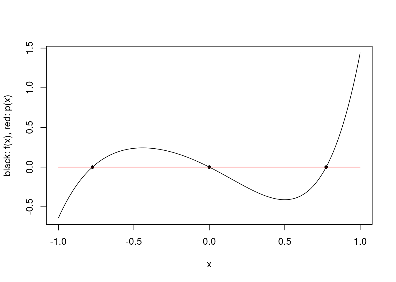
The approximating polynomial is the zero polynomial, simply because \(p_3\) is \(0\) at the interpolation points by construction. While this is a poor approximation of the function, the integral of \(p_3 q\) over \([-1,1]\) is \(0\) so their integrals are the same. Finally, we can superimpose the function \(r\) over the polynomial approximation of \(f\), and we see that indeed the polynomial approximation is exactly \(r\).
plot.polynomial.approximation(f, pts, -1, 1)
vs <- seq(-1,1,0.01)
lines(vs, r(vs), col="blue", lty="dashed")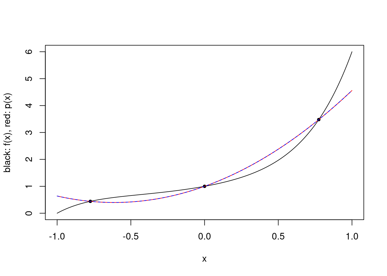
In the case where \(w \equiv 1\), for a given \(k\) one has \[\hat{I}_{\rm Gauss-Legendre}(f) = \frac{(b-a)^{2k+1}(k!)^4}{(2k+1)\{(2k)!\}^3} f^{(2k)}(\xi),\] for some \(\xi \in (a,b)\). For a composite Gauss–Legendre rule, one obtains \[\hat{I}^m_{\rm Gauss-Legendre}(f) = \frac{(b-a)^{2k+1}(k!)^4}{m^{2k}(2k+1)\{(2k)!\}^3} f^{(2k)}(\xi),\]
We can now add the errors for composite Gauss–Legendre quadrature (\(k \in \{3,4,5\}\)) to the previous plot for composite Newton–Cotes rules, with \(f=\sin\) and \((a,b) = (0,10)\). When the mathematical error for these rules is close to or less than \(10^{-15}\), the numerical error starts to be dominated by roundoff error, and so the results are not plotted.
gauss.legendre.canonical <- function(f, k) {
  if (k == 1) {
    return(2*f(0))
  }
  if (k == 2) {
    return(f(-1/sqrt(3)) + f(1/sqrt(3)))
  }
  if (k == 3) {
    return(5/9*f(-sqrt(3/5)) + 8/9*f(0) + 5/9*f(sqrt(3/5)))
  }
  if (k == 4) {
    tmp <- 2/7*sqrt(6/5)
    xs <- rep(0, 4)
    xs[1] <- sqrt(3/7 - tmp)
    xs[2] <- -sqrt(3/7 - tmp)
    xs[3] <- sqrt(3/7 + tmp)
    xs[4] <- -sqrt(3/7 + tmp)
    ws <- rep(0, 4)
    ws[1] <- ws[2] <- (18+sqrt(30))/36
    ws[3] <- ws[4] <- (18-sqrt(30))/36
    return(sum(ws*vapply(xs, f, 0)))
  }
  if (k == 5) {
    tmp <- 2*sqrt(10/7)
    xs <- rep(0, 4)
    xs[1] <- 0
    xs[2] <- 1/3*sqrt(5 - tmp)
    xs[3] <- -1/3*sqrt(5 - tmp)
    xs[4] <- 1/3*sqrt(5 + tmp)
    xs[5] <- -1/3*sqrt(5 + tmp)
    ws <- rep(0, 5)
    ws[1] <- 128/225
    ws[2] <- ws[3] <- (322 + 13*sqrt(70))/900
    ws[4] <- ws[5] <- (322 - 13*sqrt(70))/900
    return(sum(ws*vapply(xs, f, 0)))
  }
  stop("not implemented")
}

gauss.legendre <- function(f, a, b, k) {
  g <- change.domain(f, a, b, -1, 1)
  gauss.legendre.canonical(g, k)
}
composite.gauss.legendre <- function(f, a, b, subintervals, k) {
rule <- function(f, left, right) {
gauss.legendre(f, left, right, k)
}
return(composite.rule(f, a, b, subintervals, rule))
}
composite.gl.3 <- vapply(ms, function(m) composite.gauss.legendre(sin, 0, 10, m, 3), 0)
composite.gl.3[log(abs(composite.gl.3 - val)) < -33] <- NA
composite.gl.4 <- vapply(ms, function(m) composite.gauss.legendre(sin, 0, 10, m, 4), 0)
composite.gl.4[log(abs(composite.gl.4 - val)) < -33] <- NA
composite.gl.5 <- vapply(ms, function(m) composite.gauss.legendre(sin, 0, 10, m, 5), 0)
composite.gl.5[log(abs(composite.gl.5 - val)) < -33] <- NA
tg3 <- tibble(m=ms, rule="gauss-legendre 3", log.error=log(abs(composite.gl.3- val)),
theory=log(0.18*factorial(3)^4/factorial(2*3)^3/(2*3+1)*10^7/ms^6))
tg4 <- tibble(m=ms, rule="gauss-legendre 4", log.error=log(abs(composite.gl.4- val)),
theory=log(0.18*factorial(4)^4/factorial(2*4)^3/(2*4+1)*10^9/ms^8))
tg5 <- tibble(m=ms, rule="gauss-legendre 5", log.error=log(abs(composite.gl.5- val)),
theory=log(0.18*factorial(5)^4/factorial(2*5)^3/(2*5+1)*10^11/ms^10))
tib <- bind_rows(tr, tt, tm, ts, tg3, tg4, tg5)
ggplot(tib, aes(x=m, colour=rule)) + geom_point(aes(y=log.error), na.rm=TRUE) + geom_line(aes(y=theory))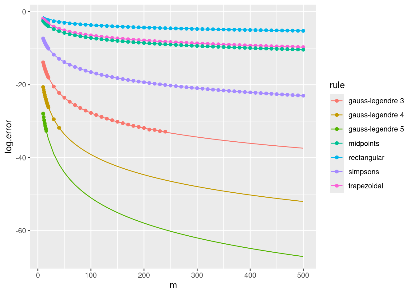
The Gauss–Legendre rule for \(k=1\) is equivalent to the midpoint rule, and the Gauss–Legendre rule for \(k=2\) is very similar to Simpson’s rule in terms of error. However, with \(k=3\) we begin to see a dramatic improvement due to the much faster rate of convergence.
Practical algorithms
We have a seen a few simple numerical integration rules that all arise by integrating an interpolating polynomial defined by specific interpolation points. In practice, these types of rules are popular, but are enhanced by various types of adaptation and practical error estimation.
Specifically, algorithms are designed to provide an approximation of any integral to a given precision. In order to do this effectively, estimates or bounds on the error need to be computed. In order to reduce overall computational cost, it is also sensible to define algorithms that spend relatively more computational effort in subintervals where the integral is estimated poorly. Similarly, defining a robust algorithm can also involve specifying appropriate change of variables formulas for dealing with semi-infinite and infinite intervals, and techniques for dealing with singularities. One can also obtain performance improvements though the choice of weight function in the general weighted integration problem \(I(f) = I_w(g) = \int g(x) w(x) {\rm d}x\): by choosing an easily integrable \(w\) appropriately, \(g\) may be better approximated by a polynomial.
Multiple integrals
We have seen that one-dimensional integrals of sufficiently smooth functions on a finite domain \([a,b]\) can be approximated to arbitrary accuracy with relatively small computational cost. We consider now only a very simple approach to multiple integrals. Consider an integral over \(D = [a_1,b_1] \times \cdots \times [a_d,b_d]\).
\[I(f) = \int_D f(x_1,\ldots,x_d) {\rm d}(x_1,\ldots,x_d).\]
Appealing to Fubini’s Theorem, and letting \(D' = [a_2,b_2] \times \cdots \times [a_d,b_d]\) we can often rewrite \(I(f)\) as an iterated integral
\[I(f) = \int_{a_1}^{b_1} \int_{D'} f(x_1,\ldots,x_d) {\rm d}(x_2,\ldots,x_d) {\rm d}x_1 = \int_{a_1}^{b_1} g(x_1) {\rm d}x_1,\] where taking \(h_{x_1}(x_2,\ldots,x_d) = f(x_1,\ldots,x_d)\) we have \[g(x_1) = I(h_{x_1}) = \int_{D'} h_{x_1}(x_2,\ldots,x_d) {\rm d}(x_2,\ldots,x_d).\]
Recursive algorithm
It is natural to define a recursive algorithm whereby one uses an approximation of \(g\) obtained by numerical integration to approximate \(I(f)\). That is, we use the one-dimensional quadrature rule
\[\hat{I}(f) = \sum_{i=1}^k \hat{g}(x_1^{(i)}) \int_{a_1}^{b_1} \ell_i(x_1) {\rm d}x_1,\]
where \(\hat{g}(x_1) = \hat{I}(h_{x_1})\).
We implement this recursive algorithm in R, using the Gauss–Legendre (k=5) rule for every one-dimensional integral.
# approximates multiple integrals using nested composite Gauss--Legendre (k=5)
# f should take a vector of length d as input, and as and bs should be the lower
# and upper limits of integration
my.integrate <- function(f, as, bs, subintervals) {
  stopifnot(length(as) == length(bs))
  d <- length(as) # dimension is length of limit vectors
  if (d == 1) {
    # just integrate the 1D function
    return(composite.gauss.legendre(f, as, bs, subintervals, 5))
  } else {
    # define a 1D function obtained by (approximately) integrating x_2,...,x_d
    g.hat <- function(x) {
      my.integrate(function(y) f(c(x,y)), as[2:d], bs[2:d], subintervals)
    }
    # integrate g.hat
    return(composite.gauss.legendre(g.hat, as[1], bs[1], subintervals, 5))
  }
}
We can test out the algorithm on a slightly challenging three-dimensional integral. Specifically, the \(\sin\) function cannot be approximated well by a degree 9 polynomial over \([0, 8\pi + 3\pi/2]\), so a few subintervals are required to give accurate answers.
f <- function(x) {
  sin(sum(x))
}

# actual value is 2
vapply(1:7, function(m) my.integrate(f, rep(0,3), rep(8*pi+3*pi/2,3), m), 0)
## [1] 705.074761 7.045259 1.932086 1.993652 2.002155 2.000079 2.000011The curse of dimensionality
As in the one-dimensional case, numerical integration via polynomial interpolation can in principle provide very accurate approximations for sufficiently smooth functions. However, the computational cost of the algorithm grows rapidly with dimension.
Although we have defined the multiple integral algorithm recursively, to take advantage of existing functions, one can also see that its multiple integral, or “cubature”, rule is of the form
\[\hat{I}(f) = \sum_{i=1}^{n} w_i f(x_i),\]
where the points \(x_1,\ldots,x_n\) are arranged in \(d\)-dimensional space. The my.integrate function arranges \(n = (mk)^d\) points in a regular grid. One can clearly see that for fixed \((m,k)\), the computational cost is exponential in \(d\) and so quickly becomes prohibitive as \(d\) increases.
One may wonder if the curse of dimensionality is specific to regular grids, as indeed there are better rules that use irregular grids. However, there are certainly classes of functions that require exponential in \(d\) computational time; see, e.g. a recent survey of complexity results.
It is clear that the smoothness of \(f\) is important for the quadrature rules that we have considered. From the survey linked above, we can see that for \(r \in \mathbb{N}\), the class of \(C^r([0,1]^d)\) functions with all partial derivatives bounded by 1 does suffer from the curse. However, an outstanding open problem is whether the class of \(C^\infty([0,1]^d)\) functions with all partial derivatives bounded by 1 suffers from the curse. For a smaller class of infinitely differentiable functions, the curse does not hold. See also this recent paper for some recent progress on integration schemes with optimal convergence rates.
When one requires an approximation of a high-dimensional integral in many statistical applications, one often resorts to Monte Carlo methods as they do not suffer from the curse of dimensionality in the same way as the quadrature rules we have seen here.