Why parallel?

Often, for large data processing jobs, a single CPU core is not enough. Large computational jobs can be:

• cpu-bound: takes too much cpu time
• memory-bound: takes too much memory
• I/O-bound: takes too much time to read/write from disk
• network-bound: Takes too much time to transfer across network

Parallel programming aims to distribute cpu-bound computations to different cores (in a single processor) or processors (if available). Modern supercomputers are fast because they have massive number of processors, therefore it is crucial to be able write programs that run in parallel if one wants to take advantage of large clusters of processors.

However, it is not true, even for easily parallelisable computations, that running on \(n\) processes will be \(n\) times as fast. The achievable gain using additional processors tend to diminish as \(n\) increases.

Parallelise using mclapply

library(parallel)
num_cores <- detectCores()
num_cores

## [1] 4

In a Wright-Fisher model, an important model in population genetics, we trace the frequency of a mutant in a population of constant size \(N\). The number of mutants \(X_k\) is a Markov process that depends only on the value of \(X_{k-1}\): \[ X_k | X_{k-1} \sim Binomial(N, \frac{X_{k-1}} N). \]

simulate_wright_fisher <- function(N, n_gen, init_freq) {
  # population size, number of generation to simulate, and initial frequency of mutant
  counts <- numeric(n_gen)
  counts[1] <- round(N * init_freq)
  for (k in 2:n_gen) {
    counts[k] <- rbinom(1, size=N, prob=counts[k-1]/N)
  }
  return(counts)
}
counts <- simulate_wright_fisher(5000, 10000, 0.2)
plot(counts, type='l', main='frequency of mutant', xlab='generation', ylab='')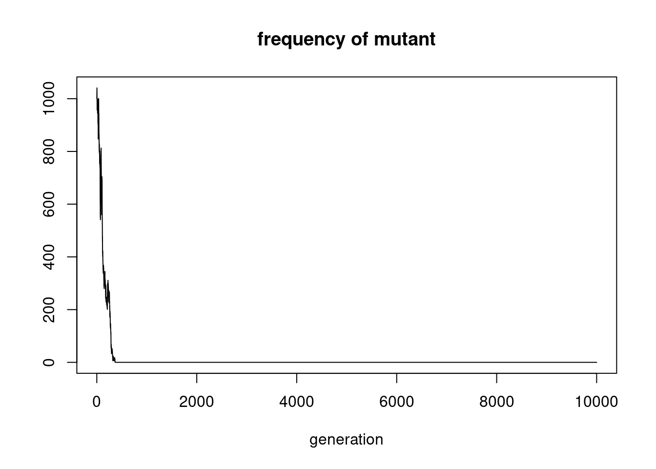

system.time(simulate_wright_fisher(5000, 10000, 0.2))

##    user  system elapsed 
##   0.019   0.004   0.023

This simple “neutral” Wright-Fisher model can still be vectorised relatively easily, but more complicated models won’t be. This is where parallelisation comes in.

mclapply() (doesn’t work on windows)

wrapper <- function(init_freq) simulate_wright_fisher(5000, 10, init_freq)
init_freqs <- rep(0.2, 3)
res <- mclapply(init_freqs, wrapper, mc.cores=2)
res

## [[1]]
##  [1] 1000 1013 1025 1044 1064 1060 1048 1063 1054 1043
## 
## [[2]]
##  [1] 1000 1013 1004 1030 1004  991 1016 1048 1026  973
## 
## [[3]]
##  [1] 1000  970  979  959  913  924  904  904  929  885

wrapper2 <- function(init_freq) tail(simulate_wright_fisher(5000, 1000, init_freq), 1)
init_freqs2 <- rep(0.2, 500)
system.time(lapply(init_freqs2, wrapper2))

##    user  system elapsed 
##   0.987   0.016   1.004

system.time(mclapply(init_freqs2, wrapper2, mc.cores=2))

##    user  system elapsed 
##   0.002   0.004   0.555

system.time(mclapply(init_freqs2, wrapper2, mc.cores=4))

##    user  system elapsed 
##   0.000   0.013   0.534

The results show that mclapply with 2 cores is twice as fast as lapply. Increasing to 4 cores improves the performance of mclapply further, but by a factor slightly less than 2. (Note that on this MacBook, there are 4 physical cores, 8 virtual cores.)

foreach and doParallel

Note that foreach is not a parallel for loop. It resembles a function that outputs something, typically a list of the same length as the number of iterates, with usage illustrated below. Note that %do% evaluates the expression sequentially, while %dopar% evaluates it in parallel.

library(foreach)
foreach (i=1:3) %do% {
  i*i
}

## [[1]]
## [1] 1
## 
## [[2]]
## [1] 4
## 
## [[3]]
## [1] 9

res <- foreach (i=1:2, .combine=rbind) %do% {
  simulate_wright_fisher(5000, 10, 0.2)
}
res

##          [,1] [,2] [,3] [,4] [,5] [,6] [,7] [,8] [,9] [,10]
## result.1 1000  975  955  927  909  919  929  902  936   903
## result.2 1000  933  884  908  905  916  934  904  919   893

A useful argument to add to foreach is .final, which is function of one argument that is called to return final. For sample, if we are only interested in the number of mutants in the most recent generation,

n_gen <- 1000
res <- foreach (i=1:1000, .combine=rbind, .final=function(x) x[,n_gen]) %do% {
  simulate_wright_fisher(5000, n_gen, 0.2)
}
hist(res, breaks=50)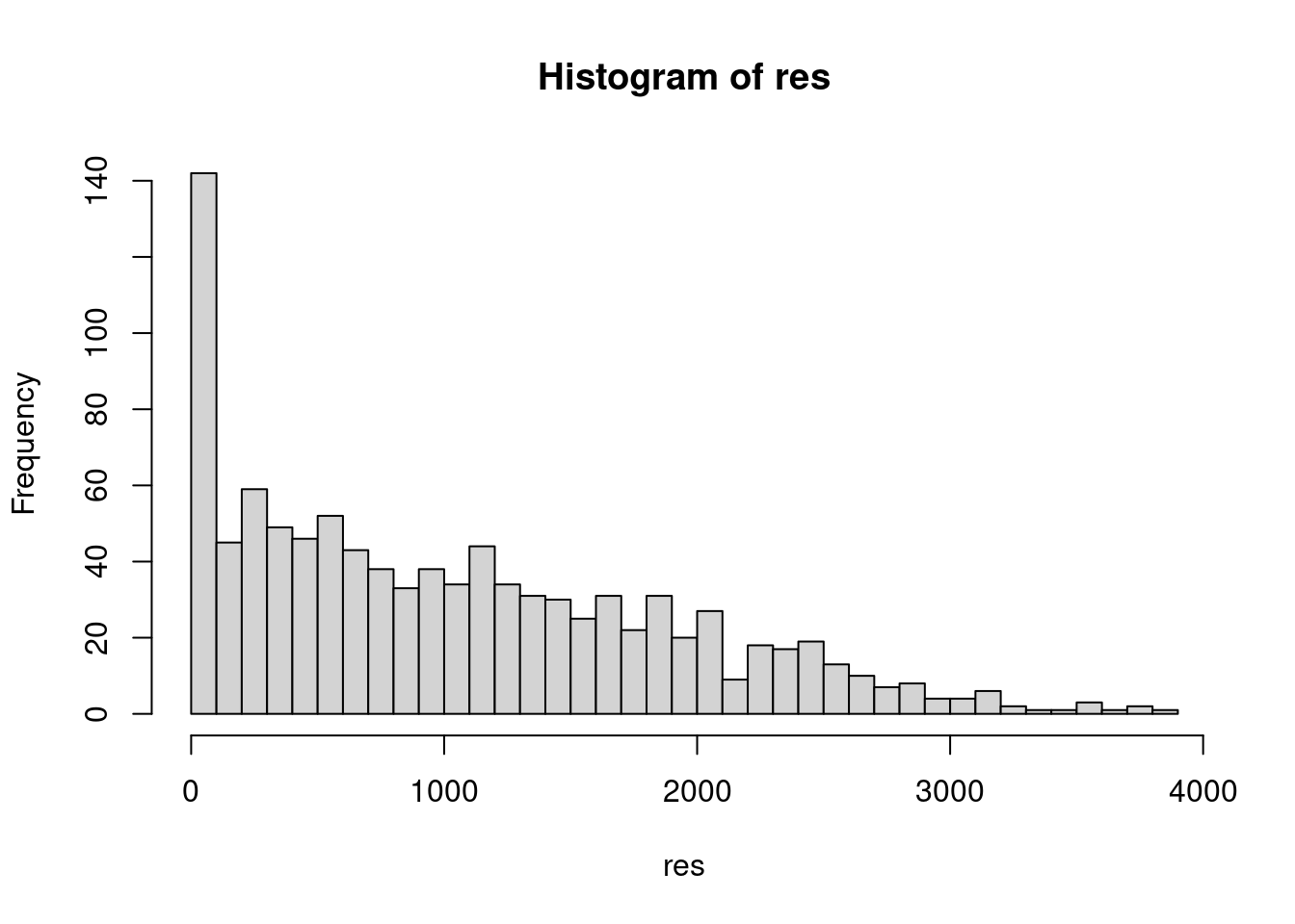

So far nothing has run in parallel. In order to do so, we need to register the number of cores to use via registerDoParallel.

library(doParallel)

## Loading required package: iterators

registerDoParallel(2) # only register 2 cores
n_runs <- 200
system.time(foreach (i=1:n_runs, .combine=rbind, .final=function(x) x[,n_gen]) %do% {
  simulate_wright_fisher(5000, n_gen, 0.2)
})

##    user  system elapsed 
##   0.436   0.000   0.437

system.time(foreach (i=1:n_runs, .combine=rbind, .final=function(x) x[,n_gen]) %dopar% {
  simulate_wright_fisher(5000, n_gen, 0.2)
})

##    user  system elapsed 
##   0.428   0.148   0.297

t1 <- Sys.time()
res1 <- foreach (i=1:n_runs, .combine=rbind, .final=function(x) x[,n_gen]) %do% {
  simulate_wright_fisher(5000, n_gen, 0.2)
}
t2 <- Sys.time()
res2 <- foreach (i=1:n_runs, .combine=rbind, .final=function(x) x[,n_gen]) %dopar% {
  simulate_wright_fisher(5000, n_gen, 0.2)
}
t3 <- Sys.time()
registerDoParallel(4) # try registering all 4 cores
res2 <- foreach (i=1:n_runs, .combine=rbind, .final=function(x) x[,n_gen]) %dopar% {
  simulate_wright_fisher(5000, n_gen, 0.2)
}
t4 <- Sys.time()

t2-t1

## Time difference of 0.4643681 secs

t3-t2

## Time difference of 0.2935133 secs

t4-t3

## Time difference of 0.3021364 secs

# clean up the cluster
stopImplicitCluster()

Just as in the case of mclapply, evaluating the code in parallel with 2 cores takes about half as much time as evaluating the code sequentially, but with 4 cores, the speedup deteriorates somewhat.