First-class functions

Perhaps the most important feature is that R has first-class functions. While most programming languages involve defining functions or procedures, a language has first-class functions if in addition:

• functions can be arguments to other functions
• functions can be returned by functions
• functions can be stored in data structures.

Essentially, functions are like any other variable.

You have already seen some functional features of R, such as the Map and Reduce functions, which take functions as arguments.

square <- function(x) x*x

unlist(Map(square, 1:5))

## [1]  1  4  9 16 25

Reduce(`+`, Map(square, 1:5), init=0)

## [1] 55

One can also return functions.

negate <- function(f) {
  function(...) {
    return(-f(...))
  }
}

negative.add <- negate(`+`)
negative.add(1, 2)

## [1] -3

Functions can be stored in lists.

arithmetic <- list(add=function(x,y) x+y, multiply=function(x,y) x*y)
arithmetic$add(1,2)

## [1] 3

Pure functions

In functional programming, one often aims to avoid functions that have side effects. That is, functions that modify global program state.

A function that always gives the same output for the same arguments and does not have any side effects is a pure function. These are very similar to mathematical functions and can be easier to reason about.

Typically, a few functions in data analysis software will need to be impure. For example, functions that perform I/O or generate pseudo-random numbers. The former is necessary to access data and/or report results.

Closures

When a function foo is created by another function make.foo, the environment in which it is created is used to resolve free variables (not arguments or locally declared) in foo. If foo has such free variables, and the environment binds them then foo is a closure.

This may sound complicated, but operationally the important feature is that functions created in an environment have access to the variables defined in that environment.

make.foo <- function(x) {
  foo <- function(y) x + y
}

f <- make.foo(10) # f(y) = 10 + y
f(3)

## [1] 13

f(5)

## [1] 15

exists('x')

## [1] FALSE

You may have used this feature without even thinking about it very much.

It is quite useful in data analysis. For example, imagine a linear regression model with design matrix \(X\) and data \(y\). One can write a function that returns a predictor, as follows.

make.predictor <- function(X, y) {
  beta <- as.vector(solve(t(X)%*%X, t(X)%*%y))
  predictor <- function(x) as.vector(x%*%beta)
}

We can check that the predictions are reasonable.

# make a "training" dataset
X <- cbind(1, matrix(rnorm(100*2), 100, 2))
beta.true <- rnorm(3)
y <- X%*%beta.true + rnorm(100)

# create the prediction function
f <- make.predictor(X, y)

# make a "testing" dataset
test.X <- cbind(1, matrix(rnorm(10*2),10,2))

# plot the true means
plot(test.X%*%beta.true, col="red", pch=20,
  main="true and predicted means for test data",
  xlab="test index", ylab="y")
# and also the predicted means
points(f(test.X), col="blue", pch=20)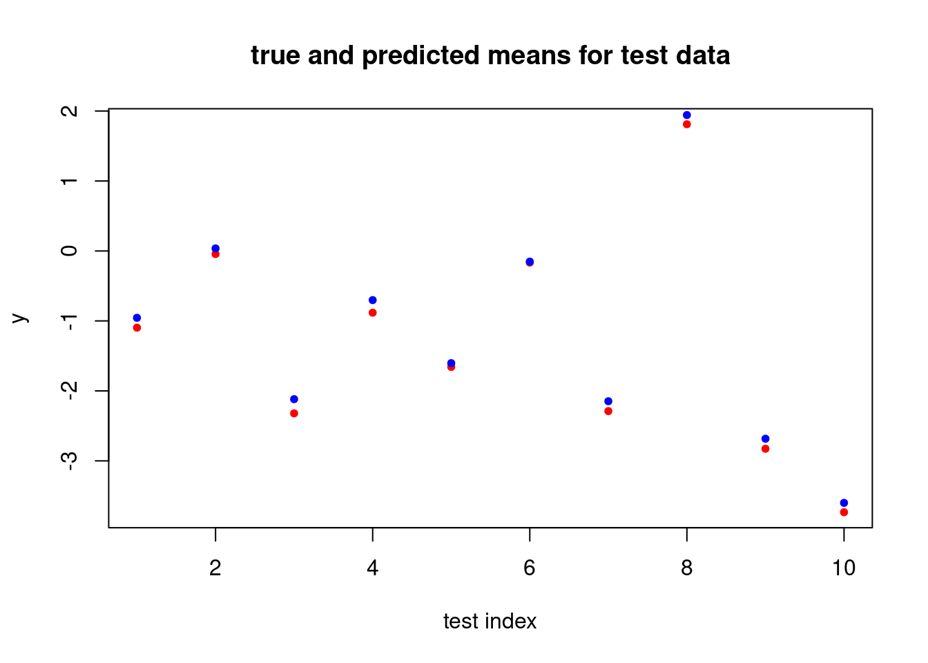

The important feature is that the estimated coefficient vector is captured by the closure. In some sense, the predictor function carries data along with it: one does not need to pass in the original data or the estimated coefficients to the predictor function. This can allow very simple interfaces to functions that are quite complicated.

The idea of closures carrying data along with functions can be thought of as an alternative to objects providing an interface to data and methods in object-oriented programming.

Note. One fairly common source of bugs is capturing the wrong variable. For example, unintentionally referring to a global variable rather than a local variable due to a spelling mistake.

Lazy evaluation

R uses lazy evaluation for function arguments, and this can cause confusion in some specific settings. This example from Advanced R is instructive.

foo <- function(x) {
  return(10)
}
foo(warning("this warning is not shown"))

## [1] 10

We can use the force function to force evaluation of an argument.

bar <- function(x) {
  force(x)
  return(10)
}
bar(warning("this warning is shown"))

## Warning in force(x): this warning is shown

## [1] 10

Lazy evaluation is useful because it can reduce the number of times expressions are evaluated. But it may be difficult to reason about, especially when dealing with functions that return functions. Consider another example from Advanced R.

make.power.function <- function(exponent) {
  power <- function(x) x^exponent
}

square <- make.power.function(2)
cube <- make.power.function(3)

square(3)

## [1] 9

cube(3)

## [1] 27

The following is probably not what you expected, however.

exponent <- 2
square <- make.power.function(exponent)
exponent <- 3
square(2)

## [1] 8

What has happened is that exponent is only lazily evaluated when square is called, at which point exponent = 3.

To fix the “bug”, one can force the evaluation of exponent in make.power.function.

make.power.function <- function(exponent) {
  force(exponent)
  power <- function(x) x^exponent
}
exponent <- 2
square <- make.power.function(exponent)
exponent <- 3
square(2)

## [1] 4