Object-oriented programming

Outlook
Terminology
S3
S4
Reference Classes

Outlook

The purpose of this chapter is to introduce object-oriented programming (OOP) in R. Base R offers three different models for OOP:

Further, some R packages on CRAN are available that provide additional models (e.g., R6, R.oo or proto).

Here we focus on an introduction of the models available in base R and a discussion of their advantages and disadvantages. For a more in-depth introduction to the mechanics of OOP in R you may want to read in Part III of Advanced R.

Terminology

An important reason to use OOP is that it allows for polymorphism, which greatly facilitates re-usability and extendability. Polymorphism means that a single symbol may refer to different types. In particular, this approach allows for the separation of the interface of a piece of software and its implementation. A software developer who wants to reuse some already existing software thus only needs to know the interface against which he is programming and what the expected behaviour is. The details of the implementation on the other hand are not required to be known. One specific implementation of an interface could thus even be exchanged for another one and the two implementations may (internally) works quite different without affecting the validity of the software that makes use of them.

In OOP the implementation is encapsulated in an object; i.e., its data and functionality are conceptually at the same place, but separate from the rest. The state (this can include data) of an object is specified via its fields and the behaviour is specified by its methods. Many OOP model (but not all) allow for inheritance when defining new classes. If one class (the derived class is usually referred to as the child) inherits from another class (the base class is usually referred to as the parent) then the child class will have all the fields and methods of the parent class available and the fields and methods from the definition are added to those. The resulting hierarchical structure is often displayed graphically in form of a class diagram which are part of the Unified Modelling Language (UML). The use of UML can be very helpful when designing software systems using OOP.

With classes and their relationships to each other laid out in a tactical way (e. g., via inheritance and how they interact or are associated to each other) software systems become more easily maintainable and it is often possible to extend functionality without changes to the already existing code. Reusable solutions and best practices in OOP are documented in a formalised fashion as design patterns.

The different OOP models in R vary in the degree of encapsulation that they provide. S3 is probably the least rigorous of the models available in base R. In Advanced R it is described as functional OOP, because of the mechanism in which a function call of the form generic(object, additional_args) is dispatched. Here, a method dispatch refers to finding the right code to evaluate given the type of object. S4 enforces more disciplined programming by requiring formal definitions that S3 does not require. The upside to this extra work is that a greater degree of integrity can be guaranteed. Reference Classes implement properly encapsulated object-oriented paradigm. In particular, they are mutable, meaning that they can be modified in place avoiding R’s usual copy-on-modify mechanism.

S3

The easiest and most informal system for OOP in R is called S3 (named after version 3 of the S programming language into which it was introduced). For S3 there is no formal class definition. While, on the one hand, this makes using the system very flexible, on the other hand, it also means that there are usually no build-in integrity checks. Programming with S3 is largely based on conventions. We outline how to use S3 in the rest of this section.

An S3 object is an object of a base type with the attribute class set to the class name. If you feel that you need to revise what base types and attributes are in R we refer you to Sections 3.3 and 12 in Advanced R. The functions class() and unclass() provide a convenient way to set the attribute to a class name or strip it off the object again.

It is good practice to have a constructor function that a user can call to initialise all relevant elements of the object and then return the object afterwards. In Advanced R it is recommended to have only the essential elements in the constructor and validate the arguments in a separate function (the validator). Further, in Advanced R it is recommended to have a helper function that is intended for end users. This function is meant to make the constructor more user-friendly, for example, by anticipating common mistakes and correcting them on the fly.

The following code block illustrates how to construct a vector y with $n$ responses, an $n \times p$ design matrix x and the ordinary least squares estimate b into an S3 object.

# set seed for reproducibility
set.seed(123)

# define sample size, coefficients, regressor and response
n  <- 50
b0 <- c(2, -1)
x  <- rnorm(n)
y  <- b0[1] + b0[2] * x + rnorm(n)

# Constructor for `simple_lin_regression`.
#
# This function computes the ordinary least squares estimate
# for the simple linear regression E[y|x] = b0 + b1 * x.
#
# Params: y - a vector with n elements; observed responses
#         x - a vector with n elements; observed regressors
#
# Returns: an S3 object of type simple_lin_regression
#
simple_lin_regression <- function(y, x) {
  # define design matrix
  n <- length(y)
  D <- matrix(c(rep(1, n), x), ncol = 2)
  
  # compute the OLS estimate
  b <- solve(t(D) %*% D) %*% t(D) %*% y 
  
  # the object will encapsulate y, X and b
  slr <- list(response=y, regressor=x, estimate=b)
  
  # the object `slr` is declared to be an S3 object of
  # class "simple_lin_regression", by
  class(slr) <- "simple_lin_regression"
  
  return(slr)
}

sl1 <- simple_lin_regression(y, x)

One reason for organising the data and estimates in this way is that we can now implement special versions of generic methods (e. g., print and plot) that will be capable of working with this class of objects. Methods for S3 objects are defined by the following naming convention [method_name].[class_name](). For example, we can implement print and plot for our class simple_lin_regression by the following code

print.simple_lin_regression <- function(x, ...) {
  cat("head(x) =", head(x$regressor), "\n")
  cat("head(y) =", head(x$response), "\n\n")
  cat("Estimated regression: E[y|x] = b0 + b1 * x\n")
  cat("b0 = ", x$estimate[1], " and b1 = ", x$estimate[2], ".\n", sep = "")
}

plot.simple_lin_regression <- function(x, y = NULL, ...) {
  plot(x = x$regressor, y = x$response,
       xlab = expression(X), ylab = expression(Y))
  abline(a = x$estimate[1], b = x$estimate[2])
}

Now we call them on the object sl that we previously created.

print(sl1)

## head(x) = -0.5604756 -0.2301775 1.558708 0.07050839 0.1292877 1.715065 
## head(y) = 2.813794 2.201631 0.3984212 3.298094 1.644941 1.801406 
## 
## Estimated regression: E[y|x] = b0 + b1 * x
## b0 = 2.147615 and b1 = -1.035079.

plot(sl1)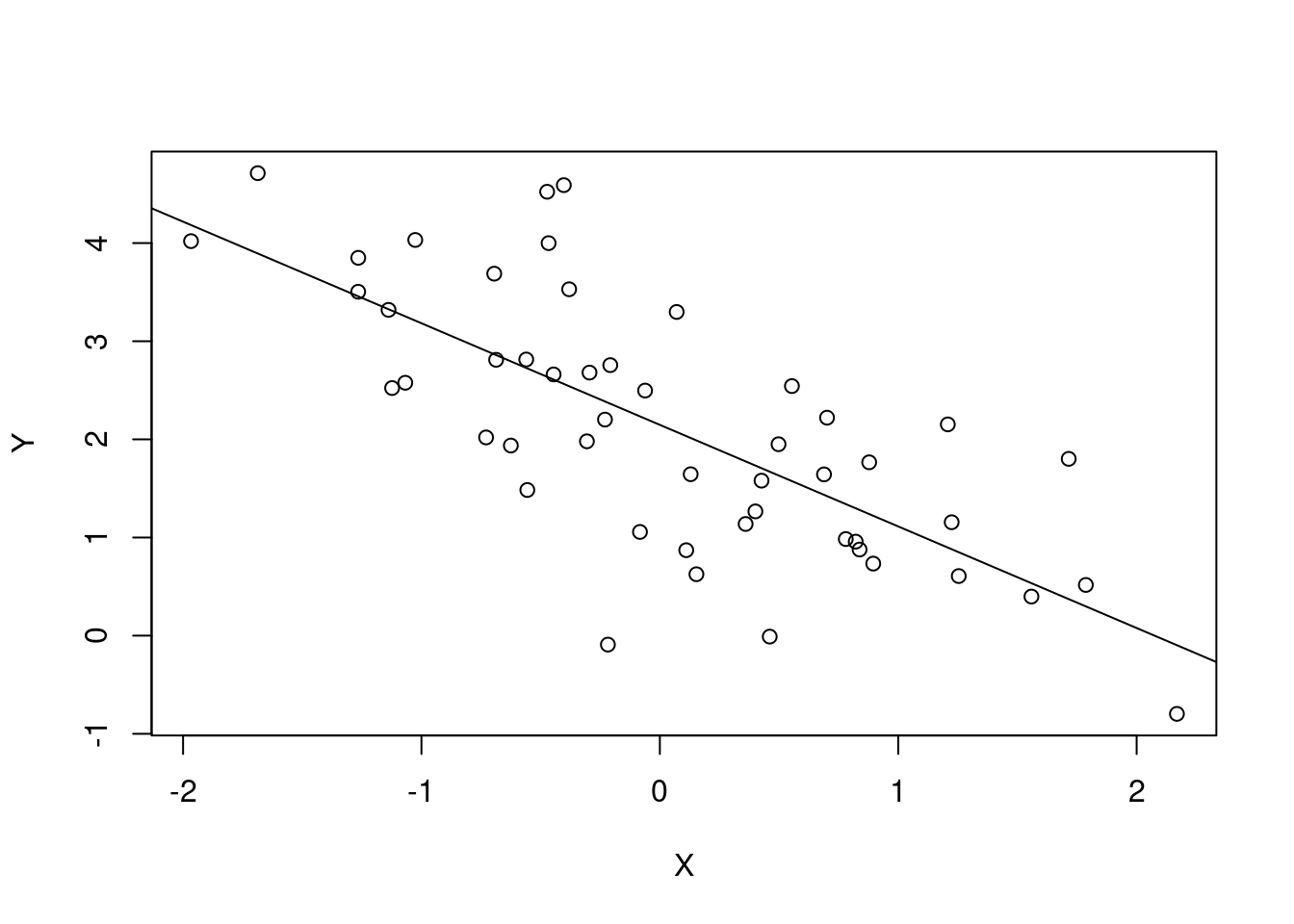

Note that to implement a method for an S3 class, a generic function of the same name needs to exist. You can, for example, see the definition of the generic function plot by

plot

## function (x, y, ...) 
## UseMethod("plot")
## <bytecode: 0x555b0ef04dc0>
## <environment: namespace:base>

Note that the generic function plot has two compulsory arguments x and y and optional arguments indicated by .... The generic functions body is always a call of the function UseMethod("[name_of_generic_function]").

When defining a method that implements a generic function for an S3 object it must have the same arguments as the generic function.

It is possible to introduce new generic functions. For example, we want to do a residual analysis. No generic residual_analysis does yet exist and we therefore define it ourselves:

residual_analysis <- function(x) {
  UseMethod("residual_analysis")
}

Next we implement it for our simple_lin_regression class:

residual_analysis.simple_lin_regression <- function(x) {
  predictions <- x$estimate[1] + x$estimate[2] * x$regressor
  plot(x = predictions, y = x$response - predictions,
       xlab = expression(hat(Y)), ylab = expression(Y - hat(Y)))
}

Now, we can apply the residual analysis function to our object:

residual_analysis(sl1)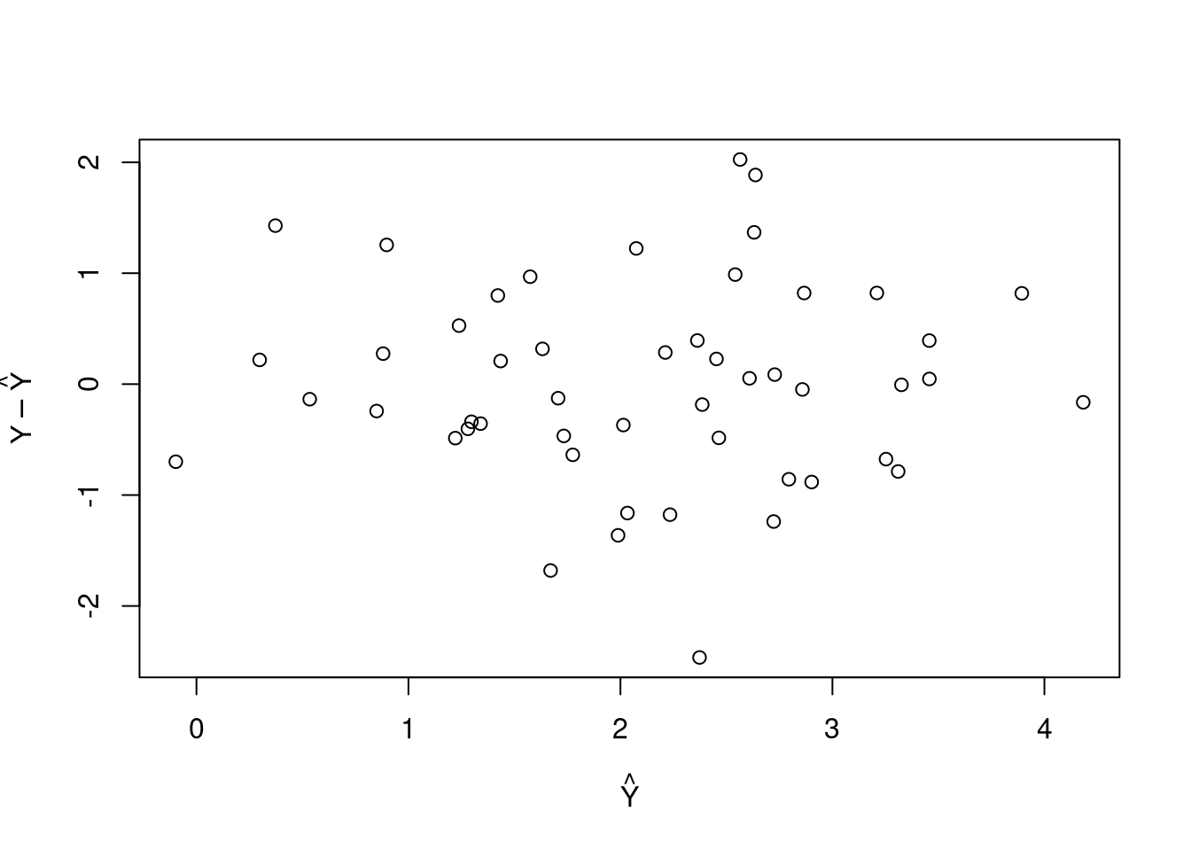

S3 classes allow for inheritance by setting the class attribute to a vector of class names.

For an example let us create an object of class ordered and check its class:

ord_factor <- ordered(c("a", "b", "a"))
class(ord_factor)

## [1] "ordered" "factor"

You can see that the first element of the class attribute is ordered and the second is factor. This means that the class ordered extends the class factor. If a generic is implemented for the class ordered it will be called, but if it is not (yet) implemented the dispatch mechanism will try to find an implementation of the generic for class factor.

Let us try this in a synthetic example:

# define objects of class parent and child, respectively.
P <- structure(numeric(), class = "parent_class")
C <- structure(numeric(), class = c("child_class", "parent_class"))

# now implement print, first for parent_class
print.parent_class <- function(x) {
  cat("this is print for parent_class objects")
}

print(P)

## this is print for parent_class objects

print(C)

## this is print for parent_class objects

# now implement print for child_class
print.child_class <- function(x) {
  cat("this is print for child_class objects")
}

print(P)

## this is print for parent_class objects

print(C)

## this is print for child_class objects

It can be seen that when the first two print statements are called (before the print method for child class is implemented) both C and P are recognised as having the functionality of the parent class. But once the print function for the child class is available C is printed as a child_class object and P is printed as a parent class object.

We stop short of explaining more details of inheritance with S3 and refer to the additional documentation.

S4

A more formal approach to OOP in R is implemented in S4 (named after version 4 of the S programming language into which it was introduced). In S4 all relevant elements as, for example, classes have to be defined explicitly. This is in sharp contrast of S3 which is largely based on conventions. While, on the one hand, this requires additional effort from the programmer, on the other hand, it can also aid to achieve more clarity and allows for build-in integrity checks. We outline how to use S4 in the rest of this section. Further information can be found in, for example, the R documentation on S4 and Section 15 of Advanced R (also see the “Learning More” section of it).

The R functions related to S4 are available in the methods package. This package is usually loaded by default. It is nevertheless, for example to indicate to someone reading the code later, advisable to load it before you start using S4:

library(methods)

As mentioned before, S4 classes have to be declared formally. This is done by invoking the setClass function. As an example, we will now redo the simple linear regression example with S4:

setClass("simple_lin_regression",
   slots = c(
     response  = "numeric",
     regressor = "numeric",
     estimate  = "numeric"
     )
)

In the call of setClass above, two arguments are provided. The first argument is the name of the class that is being defined. The second argument is slots (more commonly referred as fields or variables) which is required to be a named character vector. Note that declaring an S4 class, where fields are declared by name and type, is more rigorous than declaring a class in S3 where any base typed object can be turned into an S3 object by adding the attribute class (with the name of the S3 class) to it.

After defining the fields in a class, we need to define the methods. We should first define a special initialisation method. This method must be called initialize (note the American spelling):

setMethod("initialize", "simple_lin_regression",
  function(.Object, response, regressor) {
    .Object@response  <- response
    .Object@regressor <- regressor

    # define design matrix
    n <- length(response)
    D <- matrix(c(rep(1, n), regressor), ncol = 2)

    # compute the OLS estimate
    b <- solve(t(D) %*% D) %*% t(D) %*% response
    .Object@estimate <- as.numeric(b)
    return(.Object)
  }
)

Explanation and some remarks regarding the above definition of initialize for objects of class simple_lin_regression are in order now. We first describe the code line by line.

The first two arguments to setMethod are the name of the generic function that we are implementing (here: initialize) and the signature, i.e., the classes that some of the arguments of this function have to have for this particular implementation of the function to be invoked. initialize is a non-standard generic function that is called within the function new (which constructs a new object of this class and is called by new("simple_lin_regression", response=y, regressor=x)) and should at the least set the slots to the values provided as the arguments to new.

Our implementation above will be called if the first argument .Object, which is the class of the object created by new, is of class “simple_lin_regression”. Further (cf. the second line of the call of setMethod above), we now require that only two additional arguments are provided in the call of new("simple_lin_regression", ...): these arguments must be called response and regressor and no other argument (in particular, no estimate) must be given. You may want to take a look at the definitions of the generic function initialize and the function new.

In lines 3 and 4 of the code above we then set the values of slots response and regressor to the values that are passed to the call of new. Note that slots of an object can be accessed via the @ operator. To achieve proper encapsulation, the @ operator should only be used within method definitions, but never from outside. To allow end-users to access the value of slots, one should instead provide getter and setter methods (more on that later).

In lines 5-11 we compute the least squares estimate and in line 12 we assign the estimate to the slot estimate. An important observation to be made in line 12 is that the value of the variable b has to be cast from being a matrix to being a numeric. This is important, because the slots are all typed and assigning a matrix to a numeric without casting it before would cause an error to be thrown (try that this indeed happens).

In the last line of the definition of the new initialize method we return the object with all its slots initialised with the correct values.

Note: Implementing an initialize method for a class also provides for a convenient and reliable way to set default values to each slot. Another way to set default values is by setting the prototype argument of setClass, but the R documentation of setClass contains a remark that discourages users to do so and implement the initialize method instead.

We will also implement the print and plot method for the “simple_lin_regression” S4 class. Not that this is similar to the implementation of initialize, but possibly a bit easier:

setMethod("print", "simple_lin_regression",
  function(x) {
    cat("head(x) =", head(x@regressor), "\n")
    cat("head(y) =", head(x@response), "\n\n")
    cat("Estimated regression: E[y|x] = b0 + b1 * x\n")
    cat("b0 = ", x@estimate[1], " and b1 = ", x@estimate[2], ".\n", sep = "")
  }
)

setMethod("plot", "simple_lin_regression",
  function(x) {
    plot(x = x@regressor, y = x@response,
         xlab = expression(X), ylab = expression(Y))
    abline(a = x@estimate[1], b = x@estimate[2])
  }
)

In the above implementation of the generic functions print and plot for the signature “simple_lin_regression” note that the code is almost exactly the same as the code that we used when implementing the S3 methods, but that in S4 we use the @ operator to access the slots while in S3 we used $, because we were accessing named list elements (recall that the base type of our S3 implementation was list()).

We now instantiate an object of this class by calling the function new. Just like in most other programming languages, it is not necessary to write an additional constructor function for the S4 implementation due to the more formal and rigorous implementation of OOP with S4. Rather, we simply call the function new. We also try out the print and plot functions we have defined for the class simple_lin_regression.

n  <- 50
b0 <- c(2, -1)
x  <- rnorm(n)
y  <- b0[1] + b0[2] * x + rnorm(n)
slm1 <- new("simple_lin_regression", response=y, regressor=x)
str(slm1)

## Formal class 'simple_lin_regression' [package ".GlobalEnv"] with 3 slots
##   ..@ response : num [1:50] 3.5 2.51 2.58 1.34 2.83 ...
##   ..@ regressor: num [1:50] -0.71 0.257 -0.247 -0.348 -0.952 ...
##   ..@ estimate : num [1:2] 2.04 -1.01

print(slm1)

## head(x) = -0.7104066 0.2568837 -0.2466919 -0.3475426 -0.9516186 -0.04502772 
## head(y) = 3.498145 2.512159 2.578894 1.339166 2.832166 1.764632 
## 
## Estimated regression: E[y|x] = b0 + b1 * x
## b0 = 2.036957 and b1 = -1.007284.

plot(slm1)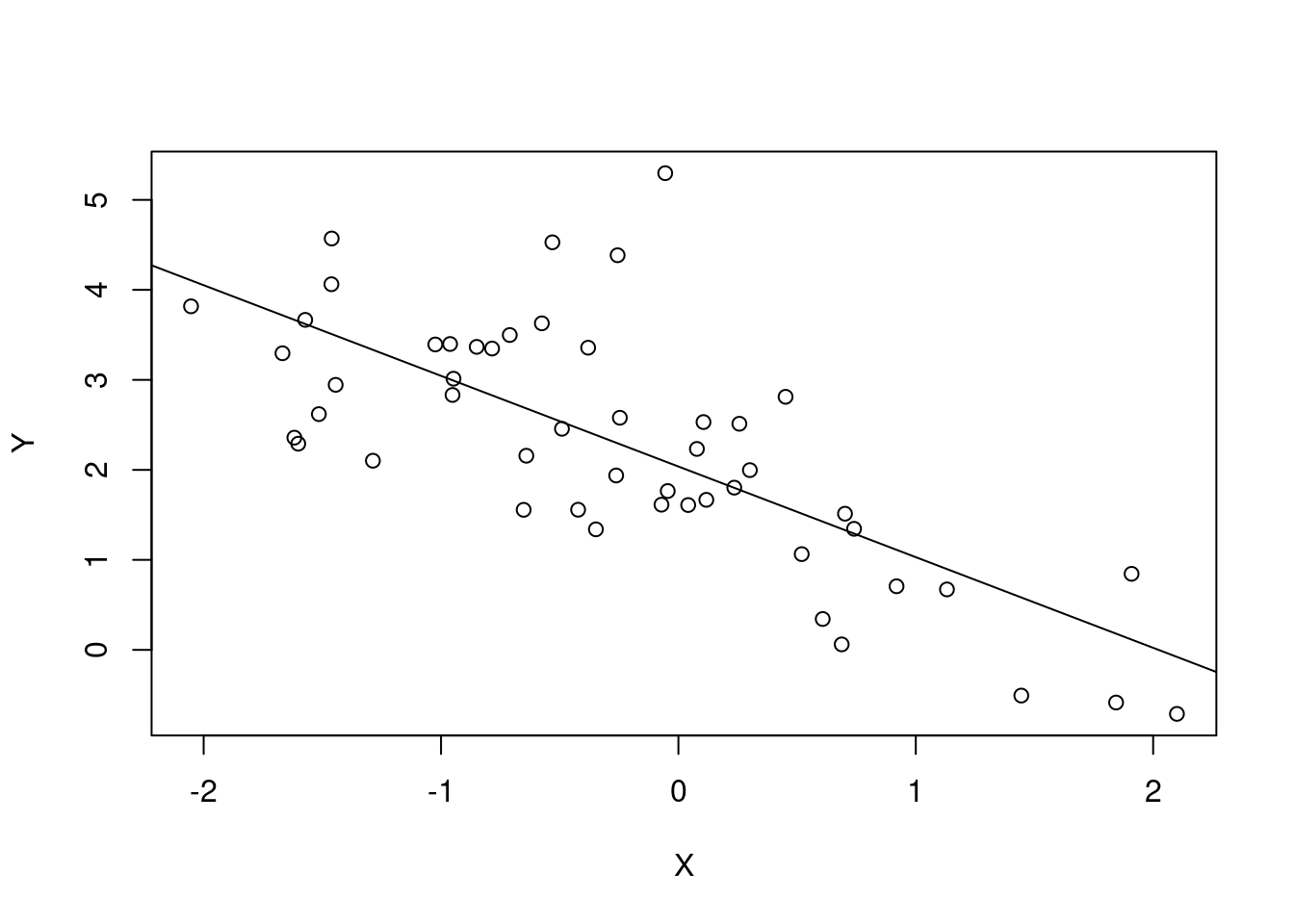

Next, we implement an S4 version of residual_analysis that we had also discussed in the chapter on S3:

setGeneric("residual_analysis")

## [1] "residual_analysis"

setMethod("residual_analysis", "simple_lin_regression",
  function(x) {
    predictions <- x@estimate[1] + x@estimate[2] * x@regressor
    plot(x=predictions, y=x@response - predictions,
         xlab=expression(hat(Y)), ylab=expression(Y - hat(Y)))
  }
)

residual_analysis(slm1)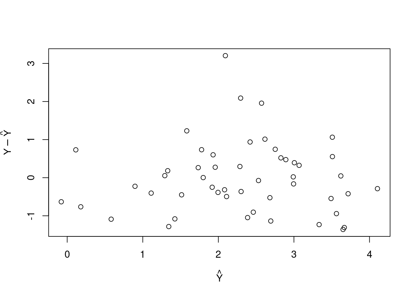

In S4, we use setGeneric to make the residual_analysis generic function available and then setMethod to implement it for objects of class simple_lin_regression. Note that we have again used the @ operator in the implementation.

Next, we will add getter and setter methods that were mentioned before. Getter and setter methods should be provided to end users when they are meant to read and write the values of slots. First we do this for the response slot:

setGeneric("response", function(x) standardGeneric("response"))

## [1] "response"

setGeneric("response<-", function(x, value) standardGeneric("response<-"))

## [1] "response<-"

setMethod("response", "simple_lin_regression", function(x) x@response)
setMethod("response<-", "simple_lin_regression",
  function(x, value) {
    x <- initialize(x, response = value, regressor = x@regressor)
    validObject(x)
    return(x)
  }
)

Note that the setter function calls the initialize function again before returning the updated object. Further, the method validObject is called before the modified object is returned. Calling validObject(x) tests if the S4 object x is formally valid. Having such a function in place is one of the build-in mechanisms that ensures integrity. We comment a bit more on it in one of the next paragraphs. Now, we can use this function to retrieve or modify the value of the response slot in the object. The following code prints the summary of the object slm1, then changes the value of the first observation of the response by adding 20 (making this observation an outlier), then print the summary of the updated object slm1:

print(slm1)

## head(x) = -0.7104066 0.2568837 -0.2466919 -0.3475426 -0.9516186 -0.04502772 
## head(y) = 3.498145 2.512159 2.578894 1.339166 2.832166 1.764632 
## 
## Estimated regression: E[y|x] = b0 + b1 * x
## b0 = 2.036957 and b1 = -1.007284.

response(slm1)[1] <- response(slm1)[1] + 20
print(slm1)

## head(x) = -0.7104066 0.2568837 -0.2466919 -0.3475426 -0.9516186 -0.04502772 
## head(y) = 23.49815 2.512159 2.578894 1.339166 2.832166 1.764632 
## 
## Estimated regression: E[y|x] = b0 + b1 * x
## b0 = 2.388623 and b1 = -1.197652.

Note that we have changed the value of the response slot, but the estimate slot was updated as well (without the end user having to do anything to make this happen).

Now we come back to the mechanism to check validity of an object. Besides the standard checks, it is possible to add further checks. For example, we might want to ensure that response and regressor are always vectors of the same length. Note that we don’t need to make sure that it is numerical vectors, because this is already ensured by the default mechanism, as the following code illustrates:

#>  response(slm1) <- "this shouldn't be text!"

##  Error in (function (cl, name, valueClass)  :
##    assignment of an object of class “character” is not valid for @‘response’
##    in an object of class “simple_linear_regression”; is(value, #"numeric")
##    is not TRUE

Next we are going to implement a validitor for our class, using the setValidity method:

setValidity("simple_lin_regression",
            function(object) {
              if(length(object@response) == length(object@regressor)) TRUE
              else paste("Unequal lengths of regressor and response.")
            })

## Class "simple_lin_regression" [in ".GlobalEnv"]
## 
## Slots:
##                                     
## Name:   response regressor  estimate
## Class:   numeric   numeric   numeric

Now, if we try to set the response slot to a numerical vector of length different to n we will see an error specific to the violation of our condition:

#>  response(slm1) <- response(slm1)[1:49]

## Error in validObject(x) :
##   invalid class “simple_lin_regression” object: Unequal lengths of regressor
##   and response.

Similarly to the response slot, we now define getter and setter methods for the regressor slot. Further, for the estimate slot we define a getter method. We do not define a setter method for the estimate slot, because end users are not supposed to change the values of estimate. The estimate is computed automatically and always corresponds to response and regressor.

setGeneric("regressor", function(x) standardGeneric("regressor"))

## [1] "regressor"

setGeneric("regressor<-", function(x, value) standardGeneric("regressor<-"))

## [1] "regressor<-"

setMethod("regressor", "simple_lin_regression", function(x) x@regressor)
setMethod("regressor<-", "simple_lin_regression",
  function(x, value) {
    x <- initialize(x, response = x@response, regressor = value)
    validObject(x)
    return(x)
  }
)

setGeneric("estimate", function(x) standardGeneric("estimate"))

## [1] "estimate"

setMethod("estimate", "simple_lin_regression", function(x) x@estimate)

Next, we test the getter and setter for the regressor slot as before, but we use the getter for the estimate slot instead of the print method:

estimate(slm1)

## [1]  2.388623 -1.197652

regressor(slm1)[1] <- regressor(slm1)[1] + 20
estimate(slm1)

## [1] 2.5684450 0.8505311

The residual plot nicely shows the outlier that we have introduced:

residual_analysis(slm1)

We are now going to (very briefly) discuss how relationships between objects can be modelled with S4. For a more depth discussion on this topic, please refer to the recommended literature.

When individual objects are related to one another this can be called an instance-level relationship. To model this kind of relationship a slot is added to the two classes of which individual objects will be related and the type of the slot will be the class of the related object.

When all objects of one class are related to all objects of another class in the way that one is a more general version of the other then we model inheritance. In S4 a class is modelled to inherit from another class by adding the contains argument to the call of setClass. If a child class inherits from a parent class this implies that the child will have all slots available that are available to the parent. S4 allows for multiple inheritance such that a vector of classes to inherit from can be provided. In this case a child has all slots of all its parents available.

The inheritance relationships also determine the behaviour of the object; i.e., which methods are associated with a class. The method dispatch (the process of determining which implementation of a generic is called) with S4 can become quite complicated when multiple inheritance or multiple arguments are present. But, if there is only one argument and no multiple inheritance it is quite straight forward to see which method is called: it is first tested whether the method is implemented for the classes of the argument and if not the parent is tested, then the “grand parent”, etc. You may want to refer to ?Methods_Details or Section 15.5 in Advanced R for details on the method dispatch in more difficult cases.

Reference Classes

While S3 and S4 are object-oriented in the sense that they provide polymorphism by the introduction of classes, generic functions and the respective method dispatch mechanism, we have also seen that encapsulation is not as consequently implemented as in other programming languages (as e.g. in C++ or Python). Reference Classes provide a model for OOP that allows for a higher degree of encapsulation where methods are not declared as generic functions and then implemented for the class, but they are implemented as part of the class definition.

Another important difference between Reference Class and S3/S4 is that it allows for modify-in-place semantics which is different from the copy-on-modify semantics that R uses in most circumstances. Note how this corresponds to more encapsulation, because it allows for the data “inside the object” to be modified by the methods of the object. We will see an example later.

Instead of re-implementing the linear model example for a third time, we are now going to discuss an artificial example. In this example we will have a class DataContainer that has a field data which holds some numbers. On generation of the object the data is set, but only when a getter method for the field result is called will some computation be performed (think of a result that is frequently needed, but very expensive to obtain; here, we compute the mean of the data which isn’t expensive, but you get the idea). After the computation is completed a flag indicating that the computation is done will be set and the result is returned. If the getter is called again, result will be returned without the computation. Unless, new data is set, which will cause flag to be reset, such that if the getter method for result is called again the computation is redone.

library(methods)

DataContainer <- setRefClass("DataContainer",
                             fields=c(data="numeric", flag="logical", result="numeric"))

DataContainer$methods(
  initialize = function(data) {
    .self$data <- data
    .self$flag <- FALSE
  },
  doComputation = function() {
    cat("MSG: doing computation now!\n")
    .self$result <- mean(.self$data)
    .self$flag   <- TRUE
  },
  show = function() {
    cat("head(data) =", head(.self$data), "\n", sep=" ")
    cat("result     =", head(.self$result), "\n", sep=" ")
  },
  getResult = function() {
    if (!flag) {
      .self$doComputation()
    }
    return(result)
  },
  setData = function(value) {
    .self$initialize(data = value)
  }
)

We now briefly comment on the code above, before we show that it indeed works how it is supposed to and compare with an analogous S4 implementation that we will see does not work as this one.

First note that the call of setRefClass is quite similar to the call of setClass when S4 was used. You can find the documentation by calling ?setRefClass. Note that the fields of the class are defined via the argument fields (in setClass for S4 they were called slots). Many further options are available, as for example declaring inheritance relationships or a mechanism to lock fields to make them private. We will not discuss these details here any further and refer you to the documentation within R. It is important to observe that the call of setRefClass returns a generator function which we assign to the variable DataContainer. In fact, setClass for S4 returns a generator function as well, but for Reference Classes it is more important to be able to access it, as can be seen now. Next we define methods of DataContainer: initialize, doComputation and show. Further, we define in the same call to methods the getter getResult and the setter setData. Note that we have not used the accessors function of the generator as this would not allow us to implement the special behaviour we would like to see. Further, note that in the definition of the functions we use .self to refer to the object from within, similar to self in e.g. Python and this in C++.

We call the new function of DataContainer to instantiate a new DataContainer object. Note that we use $ to access methods in an object, similar to . in Python or C++. We will illustrate the modify-in-place behaviour of Reference classes.

dC1 <- DataContainer$new(data=rnorm(5))

dC1             # no result set yet!

## head(data) = 2.19881 1.312413 -0.2651451 0.5431941 -0.4143399 
## result     =

dC1$getResult() # calling getResult() will compute the result

## MSG: doing computation now!

## [1] 0.6749865

dC1             # now the result is set

## head(data) = 2.19881 1.312413 -0.2651451 0.5431941 -0.4143399 
## result     = 0.6749865

dC1$getResult() # calling getResult() a second time returns the result,

## [1] 0.6749865

                # but doesn't do the computation again

# We now reset data to new numbers and then redo the above:
dC1$setData(rnorm(5))

dC1             # no result set yet!

## head(data) = -0.4762469 -0.7886028 -0.5946173 1.650907 -0.05402813 
## result     = 0.6749865

dC1$getResult() # calling getResult() will compute the result

## MSG: doing computation now!

## [1] -0.05251753

dC1             # now the result is set

## head(data) = -0.4762469 -0.7886028 -0.5946173 1.650907 -0.05402813 
## result     = -0.05251753

dC1$getResult() # calling getResult() a second time returns the result,

## [1] -0.05251753

                # but doesn't do the computation again

Now we do the same implementation with S4 and compare what happens:

setClass("DataContainer_S4",
  slots = c(data="numeric", flag="logical", result="numeric"))

setMethod("initialize", "DataContainer_S4",
  function(.Object, data){
    .Object@data <- data
    .Object@flag <- FALSE
    return(.Object)
  }
)

setGeneric("doComputation", function(x) standardGeneric("doComputation"))

## [1] "doComputation"

setMethod("doComputation", "DataContainer_S4",
  function(x) {
    cat("MSG: doing computation now!\n")
    x@result <- mean(x@data)
    x@flag   <- TRUE
    return(x)
  }
)

setMethod("show", "DataContainer_S4",
  function(object) {
    cat("head(data) =", head(object@data), "\n", sep=" ")
    cat("result     =", object@result, "\n", sep=" ")
  }
)

setGeneric("result", function(x) standardGeneric("result"))

## [1] "result"

setMethod("result", "DataContainer_S4",
  function(x) {
    if (!x@flag) {
      x <- doComputation(x)
    }
    return(x@result)
  }
)

setGeneric("data<-", function(x, value) standardGeneric("data<-"))

## [1] "data<-"

setMethod("data<-", "DataContainer_S4",
  function(x, value) {
    x <- initialize(x, data=value)
    return(x)
  }
)

dC1 <- new("DataContainer_S4", data=rnorm(5))

dC1         # no result set yet!

## head(data) = 0.1192452 0.2436874 1.232476 -0.5160638 -0.9925072 
## result     =

result(dC1) # calling getResult() will compute the result

## MSG: doing computation now!

## [1] 0.01736751

dC1         # but dC1$result is not set

## head(data) = 0.1192452 0.2436874 1.232476 -0.5160638 -0.9925072 
## result     =

We can see that the getter for result does the computation and returns the correct result. Also, the slot result is set, but due to the modification a copy of the object dC1 is generated which we never get to see, because result does not return it.

This concludes the chapter on object-oriented programming in R. It shall be pointed out, though, that only a fraction of the possibilities were covered here and that you are encouraged to conceptually design your software before you start coding with the right programming paradigm in mind.