Monte Carlo integration
Quadrature rules give excellent rates of convergence, in terms of computational cost, for one-dimensional integrals of sufficiently smooth functions. However, they quickly become prohibitively expensive in high-dimensional problems. To complement quadrature rules in low dimensions, we now consider the use of Monte Carlo algorithms in higher dimensions.
Let \((\mathsf{X},\mathcal{X})\) be a measurable space. We have a target probability measure \(\pi:\mathcal{X}\rightarrow[0,1]\) and we would like to approximate the quantity \[\pi(f):=\int_{\mathsf{X}}f(x)\pi({\rm d}x),\] where \(f\in L_{1}(\mathsf{X},\pi)=\{f:\pi(|f|)<\infty\}\). In other words \(\pi(f)\) is the expectation of \(f(X)\) when \(X \sim \pi\).
Reassuring note. You do not need to understand measure theory to understand most of what is said about Monte Carlo methodology. However, it allows us to present simple but general results that hold for both discrete distributions, continuous distributions and mixtures of the two. The terms probability measure and probability distribution are interchangeable. In most of what follows you can think of \(\int_{\mathsf{X}} f(x) \pi({\rm d}x)\) as \[\int_{\mathsf{X}} f(x) \pi(x) {\rm d}x,\] if \(X \sim \pi\) is a continuous random variable with probability density function \(\pi\) and as \[\sum_{x \in \mathsf{X}} f(x) \pi(x),\] if \(X \sim \pi\) is a discrete random variable with probability mass function \(\pi\).
From the measure-theoretic perspective we usually think of \(\pi\) in both cases as a density w.r.t. some dominating measure (e.g., Lebesgue or counting). Using the symbol \(\pi\) to denote both the probability measure and its density is technically ambiguous, but it is usually not possible to confuse the two.
Monte Carlo with i.i.d. random variables
Classical Monte Carlo is a very natural integral approximation method, justified at a high level by the strong law of large numbers.
Fundamental results
Theorem (SLLN). Let \((X_{n})_ {n \geq 1}\) be a sequence of i.i.d. random variables distributed according to \(\mu\). Define \[S_{n}(f):=\sum_{i=1}^{n}f(X_{i}),\] for \(f\in L_{1}(\mathsf{X},\mu)\). Then \[\lim_{n \to \infty}\frac{1}{n}S_{n}(f)=\mu(f),\] almost surely.
The random variable \(n^{-1} S_n(f)\), or a realization of it, is a Monte Carlo approximation of \(\mu(f)\). It is straightforward to deduce that the approximation is unbiased, i.e. \(\mathbb{E}[n^{-1}S_n(f)] = \mu(f)\).
This probabilistic convergence result does not provide any information about the random error \(n^{-1}S_n(f) - \mu(f)\) for finite \(n\). For \(f \in L_2(\mathsf{X}, \mu) = \{f: \mu(f^2) < \infty \}\), the variance of \(n^{-1}S_n(f)\) is straightforward to derive.
Proposition (Variance). Let \((X_{n})_ {n \geq 1}\) and \(S_n(f)\) be as in the SLLN, where \(f \in L_2(\mathsf{X}, \mu)\). Then \[{\rm var} \{ n^{-1} S_n(f) \} = \frac{\mu(f^2)-\mu(f)^2}{n}.\]
In fact, for \(f \in L_2(\mathsf{X}, \mu)\), the asymptotic distribution of \(\sqrt{n} \{ n^{-1} S_n(f) - \mu(f) \}\) is normal, by virtue of the Central Limit Theorem. This can be used, e.g., to produce asymptotically exact confidence intervals for \(\mu(f)\).
Theorem (CLT). Let \((X_{n})_ {n \geq 1}\) and \(S_n(f)\) be as in the SLLN, where \(f \in L_2(\mathsf{X}, \mu)\). Then \[n^{1/2} \{ n^{-1} S_n(f) - \mu(f) \} \overset{L}{\to} X \sim N(0,\mu(\bar{f}^2)),\] where \(\bar{f} = f - \mu(f)\).
Error and comparison with quadrature
The CLT allows us to deduce that for \(f \in L_2(\mathsf{X}, \mu)\), the error \(|n^{-1} S_n(f) - \mu(f)|\) is of order \(\mu(\bar{f}^2)^{1/2} n^{-1/2}\), since a standard normal random variable is within a few standard deviations of \(0\) with high probability.
This is of course very slow in comparison to quadrature rules in one dimension, where very fast rates of convergence can be attained for smooth functions. However, we can see that there is no mention of the dimension of \(\mathsf{X}\) in the result: it could be \(\mathbb{R}^d\) for a very large value of \(d\).
At a first glance, one benefit of Monte Carlo is that the \(\mathcal{O}(n^{-1/2})\) rate of convergence is independent of dimension. Naturally, this is not the whole story: in some cases the constant term \(\mu(\bar{f}^2)\) may grow quickly with dimension, in which case the curse of dimensionality is not avoided.
The other immediate observation we can make is that while the error of the quadrature rules we saw previously depends explicitly on the smoothness of the function being integrated, the error of \(n^{-1} S_n(f)\) depends explicitly on \(\mu(\bar{f}^2)\), i.e. the variance of \(f(X)\) when \(X \sim \mu\). There is no need for \(f\) to even be continuous, but it should ideally have a second moment under \(\mu\).
# set the seed to fix the pseudo-random numbers
set.seed(12345)

monte.carlo <- function(mu, f, n) {
  S <- 0
  for (i in 1:n) {
    S <- S + f(mu())
  }
  return(S/n)
}

1 - cos(1)
## [1] 0.4596977vapply(1:6, function(i) monte.carlo(function() runif(1), sin, 10^i), 0)## [1] 0.5806699 0.4621368 0.4720845 0.4581522 0.4597137 0.4596813Perfect sampling
Recall that we want to approximate \(\pi(f)\) for some \(f \in L_1(\mathsf{X}, \pi)\). The simplest case is where we can simulate random variates with distribution \(\pi\) on a computer. Then we can apply the SLLN with \(\mu = \pi\). If \(f \in L_2(\mathsf{X}, \pi)\) then the CLT characterizes asymptotically the error.
There are some ways of simulating according to \(\pi\) in special cases, e.g.,
- inverse transform,
- composition,
- special representations in terms of random variables we can simulate easily,
- other methods in, e.g., Luc Devroye’s Non-Uniform Random Variate Generation.
However, in many situations these techniques are not applicable. One general purpose algorithm for doing this when one can compute the density \(\pi\) pointwise and we can sample from another distribution that is “close” to \(\pi\) in a specific sense is rejection sampling.
Rejection sampling
Rejection sampling is a general purpose algorithm for simulating \(\pi\)-distributed random variates when one can sample \(\mu\)-distributed random variates and the ratio of densities \(\pi/\mu\) satisfies \(\sup_{x \in \mathsf{X}} \pi(x)/\mu(x) \leq M < \infty\).
Rejection sampling algorithm:
- Sample \(X \sim \mu\).
- With probability \(\frac{1}{M}\frac{\pi(X)}{\mu(X)}\) output \(X\), otherwise go back to step 1.
Theorem. The rejection sampling algorithm outputs a \(\pi\)-distributed random variable.
Proof. Let \(Y=\mathbb{I}\left(U<\frac{1}{M}\frac{\pi(X)}{\mu(X)}\right)\) where \(U\) is uniformly distributed on \([0,1]\), so \(Y\) is indeed \(1\) with probability \(\frac{1}{M}\frac{\pi(X)}{\mu(X)}\). For any \(A \in \mathcal{X}\), \[\begin{align} \Pr(X \in A \mid Y=1) &= \frac{\Pr(X\in A,Y=1)}{\Pr(Y=1)} \newline &= \frac{\int_{A}\frac{1}{M}\frac{\pi(x)}{\mu(x)}\mu(x){\rm d}x}{\int_{\mathsf{X}}\frac{1}{M}\frac{\pi(x)}{\mu(x)}\mu(x){\rm d}x} \newline &= \pi(A). \end{align}\] Hence \(X \mid (Y=1)\) is indeed distributed according to \(\pi\). □
The rejection sampling algorithm is very simple and powerful. However, we observe that the computational cost of the algorithm in terms of the number of simulations of \(\mu\)-distributed random variables is itself random. In fact, the cost is characterized by the value of \(M\).
Proposition. The number of simulations from \(\mu\) is a \({\rm Geometric}(1/M)\) random variable, and hence has expectation \(M\).
Proof. \(Y\) is an independent Bernoulli random variable in each loop of the algorithm with \[\Pr(Y=1)=\int_{\mathsf{X}}\frac{1}{M}\frac{\pi(x)}{\mu(x)}\mu(x){\rm d}x=\frac{1}{M},\] and the algorithm stops on the first trial where \(Y=1\). □
This is a simple implementation of a rejection sampler.
# simple but not numerically stable
# one should use log densities for high-dimensional problems
rejection.sample <- function(pi, mu, M) {
  while (TRUE) {
    x <- mu$sample()
    y <- runif(1) < pi(x)/mu$density(x)/M
    if (y) {
      return(x)
    }
  }
}
As an example, we use \({\rm Laplace}(0,1)\) distributed random variables to sample standard normal random variables.
laplace <- list()
laplace$sample <- function() {
  v <- rexp(1)
  ifelse(runif(1) < 0.5, v, -v)
}
laplace$density <- function(x) {
  return(0.5 * exp(-abs(x)))
}
M <- sqrt(2/pi) * exp(0.5) # worked this out theoretically

xs <- replicate(100000, rejection.sample(dnorm, laplace, M))
plot(density(xs))
vs <- seq(-5,5,0.01)
lines(vs, dnorm(vs), col="red")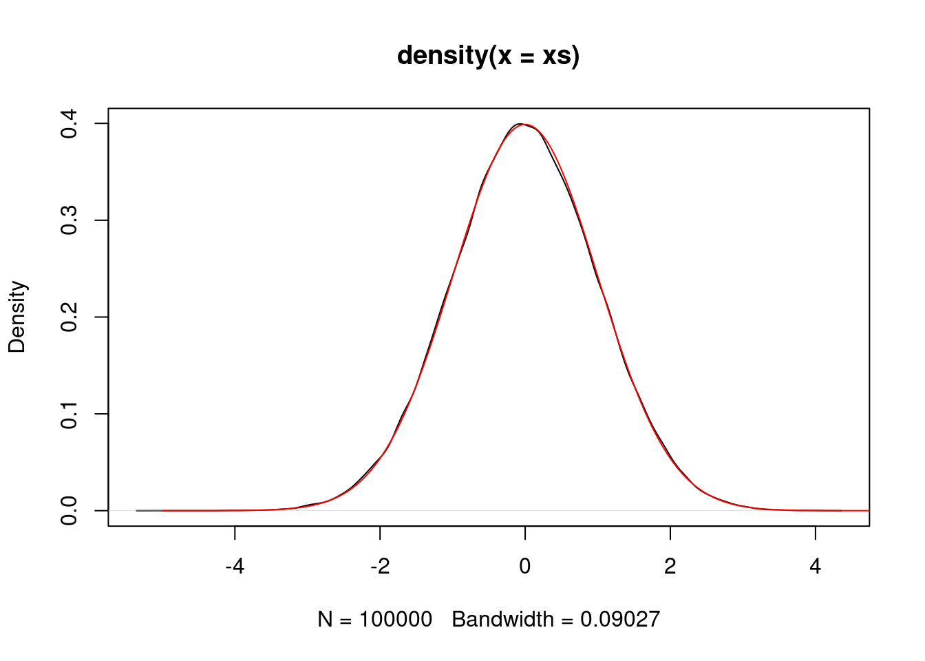
Warning. In many practical applications \(M\) is prohibitively large, and rejection sampling can easily suffer from the curse of dimensionality. For example, consider what happens as \(d\) increases when for some densities \(p\) and \(g\), \(\pi(x)=\prod_{i=1}^{d} p(x_{i})\), \(\mu(x) = \prod_{i=1}^{d} g(x_{i})\) and \(\sup_{x} \frac{p(x)}{g(x)} > 1\).
For complicated \(\pi\), especially in high dimensions, we do not usually know how to find a “good” \(\mu\).
Importance sampling
Assume \(\pi(x) > 0 \Rightarrow \mu(x) > 0\). Importance sampling is motivated by expressing \(\pi(f)\) as an integral w.r.t. \(\mu\). That is, \[\begin{align} \pi(f) &= \int_\mathsf{X} f(x) \pi({\rm d}x) \\ &= \int_\mathsf{X} f(x)w(x) \mu({\rm d}x) \\ &= \mu(f \cdot w), \end{align}\] where \(w(x) = \pi(x)/\mu(x)\) is the ratio of the densities of \(\pi\) and \(\mu\).
This justifies the use of \(n^{-1} S_n(f \cdot w)\) as an approximation of \(\pi(f)\). The variance of the approximation multiplied by \(n\) is \[\begin{align} {\rm var}(f(X)w(X)) &= \mu(\{f \cdot w\}^2) - \mu(f \cdot w)^2 \\ &= \pi(f \cdot w^2) - \pi(f)^2. \end{align}\]
In many statistical applications, importance sampling is used because it is not known how to sample \(\pi\)-distributed random variables. In such cases, it is possible that \(f \cdot w \notin L^2(\mathsf{X}, \mu)\) when \(f \in L^2(\mathsf{X}, \pi)\). A sufficient condition to ensure that \(f \in L^2(\mathsf{X}, \pi) \Rightarrow f \cdot w \notin L^2(\mathsf{X}, \mu)\) is that \(w\) is uniformly bounded.
On the other hand, importance sampling can also be used as a variance reduction technique, i.e. it is possible that \(\pi(f \cdot w^2) < \pi(f^2)\). You can try to work out what the optimal importance sampling distribution \(\mu\) in terms of minimizing the variance of the importance sampling approximation: you might consider the case where \(f\) is non-negative separately to the general case.
In high-dimensional statistical applications, it is not uncommon for the variance to be prohibitively large for reasonable values of \(n\).
importance.sample <- function(pi, mu, f, n) {
  w <- function(x) {
    return(pi(x)/mu$density(x))
  }
  fw <- function(x) {
    return(f(x)*w(x))
  }
  monte.carlo(mu$sample, fw, n)
}

# approximate the mean of a N(2,1) r.v. using Laplace(0,1) r.v.s
importance.sample(function(x) dnorm(x, mean=2), laplace, identity, 10000)
## [1] 1.930252Self-normalized importance sampling
One feature of importance sampling is that it requires the computation of \(w(x) = \pi(x) / \mu(x)\) exactly. This is problematic in cases where on can only compute \(w\) up to an unknown normalizing constant, such as in Bayesian inference where \(\pi \propto p(x)L(x)\) with \(p\) the prior and \(L\) the (observed) likelihood function.
In these cases, one can instead consider the self-normalized approximation
\[I^n_{\rm SNIS}(\pi, \mu, f) = \frac{S_n(f \cdot w)}{S_n(w)} = \frac{\sum_{i=1}^n w(X_i)f(X_i)}{\sum_{i=1}^n w(X_i)},\]
where \(X_1,X_2,\ldots\) are i.i.d. \(\mu\)-distributed random variables and \(w(x) = \pi(x)/\mu(x)\). Importantly, since \(w\) appears in both the numerator and the denominator, it can be computed up to an unknown normalizing constant. The self-normalized approximation is not unbiased in general.
As suggested above, one can view \(I^n_{\rm SNIS}(\pi, \mu, f)\) as a ratio of two importance sampling estimators. If \(\pi(x) > 0 \Rightarrow \mu(x) > 0\), one can therefore deduce that \(I^n_{\rm SNIS}(\pi, \mu, f) \to \pi(f)\) almost surely. If additionally \(\int_{\mathsf{X}}\left[1+f(x)^{2}\right]\frac{\pi(x)}{\mu(x)}\pi({\rm d}x) < \infty\) then the approximation is asymptotically normal, i.e.
\[\sqrt{n}\{I^n_{\rm SNIS}(\pi, \mu, f) - \pi(f)\} \overset{L}{\to} X \sim N(0, \sigma^2),\]
where
\[\sigma^2 = \lim_{n \to \infty} n{\rm var}(I^n_{\rm SNIS}(\pi, \mu, f)) = \int_{\mathsf{X}}\left \{ f(x)-\pi(f)\right \}^{2}\frac{\pi(x)}{\mu(x)}\pi({\rm d}x).\]
This can be proven using Slutsky’s lemma.
Notice that the asymptotic/limiting variance \(\sigma^2\) can be smaller than the corresponding asymptotic variance for importance sampling.
In high-dimensional statistical applications, it is not uncommon for the variance to be prohibitively large for reasonable values of \(n\).
sn.importance.sample <- function(pi, mu, f, n) {
  w <- function(x) {
    return(pi(x)/mu$density(x))
  }
  fw <- function(x) {
    return(f(x)*w(x))
  }
  monte.carlo(mu$sample, fw, n) / monte.carlo(mu$sample, w, n)
}

# approximate the mean of a N(2,1) r.v. using Laplace(0,1) r.v.s
# the input density for pi is multiplied by 10
sn.importance.sample(function(x) dnorm(x, mean=2)*10, laplace, identity, 10000)
## [1] 2.013923Markov chain Monte Carlo
A very powerful innovation in Monte Carlo methodology was the development of approximations involving Markov chains rather than independent random variables.
What is a Markov chain?
As before we are on a measurable space \((\mathsf{X}, \mathcal{X})\). We assume that \(\mathcal{X}\) is countably generated, e.g. the Borel \(\sigma\)-algebra on \(\mathbb{R}^{d}\). This is what “general state space” typically means in the Markov chain context.
Let \(\mathbf{X}:=(X_{n})_ {n \geq 0}\) be a discrete time Markov chain evolving on \(\mathsf{X}\) with some initial distribution for \(X_{0}\).
This means that for \(A\in\mathcal{X}\) \[\Pr\left(X_{n}\in A\mid X_{0}=x_{0},\ldots,X_{n-1}=x_{n-1}\right)=\Pr\left(X_{n}\in A\mid X_{n-1}=x_{n-1}\right),\] i.e. \(\mathbf{X}\) possesses the Markov property.
LLN and CLT
The fundamental motivation is an extension of the SLLN to the Markov chain setting. There are different versions of this kind of ergodic theorem.
Theorem (An LLN for Markov chains). Suppose that \(\mathbf{X}=(X_{n})_ {n\geq0}\) is a time-homogeneous, positive Harris Markov chain with invariant probability measure \(\pi\). Then for any \(f \in L_{1}(\mathsf{X},\pi)=\{f:\pi(\left|f\right|)<\infty\}\), \[\lim_{n\rightarrow\infty}\frac{1}{n}S_{n}(f)=\pi(f),\] almost surely for any initial distribution for \(X_{0}\).
Similarly, there are CLTs, such as the following.
Theorem (A CLT for geometrically ergodic Markov chains). Assume that \(\mathbf{X}\) is time-homogeneous, positive Harris and geometrically ergodic with invariant probability measure \(\pi\), and that \(\pi(|f|^{2+\delta})<\infty\) for some \(\delta>0\). Then \[n^{1/2} \{ n^{-1} S_{n}(f) - \pi(f) \} \overset{L}{\to} N(0,\sigma^{2}(f))\] as \(n\rightarrow\infty\), where \(\bar{f}=f-\pi(f)\) and \[\sigma^{2}(f)=\mathsf{E}_{\pi}\left[\bar{f}(X_{0})^{2}\right]+2\sum_{k=1}^{\infty}\mathsf{E}_{\pi}\left[\bar{f}(X_{0})\bar{f}(X_{k})\right]<\infty.\]
Basic definitions
The LLN and CLT we have seen make various assumptions about the Markov chain \(\mathbf{X}\) that you may not be familiar with. For this course, it is not necessary to go into too much detail about the beautiful theory underlying Markov chains on general state spaces and corresponding ergodic averages. What is clear is that we are interested in a fairly restricted set of Markov chains. So we will just define at a high-level the basic ideas.
Definition. The Markov chain \(\mathbf{X}\) is time-homogeneous if \[\Pr\left(X_{n}\in A\mid X_{n-1}=x\right)=\Pr\left(X_{1}\in A\mid X_{0}=x\right),\] for any \(n\in\mathbb{N}\).
Then \(\mathbf{X}\) is described by a single Markov transition kernel \(P:\mathsf{X}\times\mathcal{X}\rightarrow[0,1]\) with \[\Pr(X_{1}\in A\mid X_{0}=x)=P(x,A).\]
We denote by \(P^{n}\) the \(n\)-step Markov transition kernel. That is, \(P^{1}(x,A):=P(x,A)\) and \[P^{n}(x,A):=\int_{\mathsf{X}}P(z,A)P^{n-1}(x,{\rm d}z),\quad n\geq2.\]
Definition. A Markov chain \(\mathbf{X}\) has an invariant probability measure \(\mu\) if \(X_0 \sim \mu\) implies \(X_1 \sim \mu\). This is really a property of the Markov transition kernel \(P\), i.e. it means \[\mu P (A) = \int P(x, A) \mu({\rm d}x) = \mu(A), \qquad A \in \mathcal{X},\] or simply \(\mu P = \mu\).
Definition. A Markov chain is \(\varphi\)-irreducible if \(\varphi\) is a measure on \(\mathcal{X}\) such that whenever \(\varphi(A) > 0\) and \(x \in \mathsf{X}\), there exists some \(n\) possibly depending on both \(x\) and \(A\) such that \(P^{n}(x,A)>0\).
Definition. A set \(A\) is Harris recurrent if \[\Pr \left (\sum_{n=1}^{\infty}\mathbb{I}\{X_{n}\in A\} =\infty \mid X_0 = x \right ) = 1, \qquad x \in A.\]
Definition. A Markov chain is is positive Harris with invariant probability measure \(\mu\) if it is \(\mu\)-irreducible, every set \(A\in\mathcal{X}\) such that \(\mu(A)>0\) is Harris recurrent, and it has \(\mu\) as an invariant probability measure.
Definition. The total variation distance between two probability measures \(\mu\) and \(\nu\) on \(\mathcal{X}\) is \[\left\Vert \mu-\nu\right\Vert_{{\rm TV}}:=\sup_{A\in\mathcal{X}}|\mu(A)-\nu(A)|.\]
Definition. A Markov chain with invariant probability measure \(\pi\) and Markov transition kernel \(P\) is geometrically ergodic if \[\left\Vert P^{n}(x,\cdot)-\pi\right\Vert_{{\rm TV}}\leq M(x)\rho^{n},\qquad x\in\mathsf{X}\] for some function \(M\) finite for \(\pi\)-almost all \(x\in\mathsf{X}\) and \(\rho<1\).
Metropolis–Hastings
By far the most commonly used Markov chains in practice are constructed using Metropolis–Hastings Markov transition kernels. These owe their development to the seminal papers Metropolis et al. (1953) and Hastings (1970).
Algorithm
Assume \(\pi\) has a density w.r.t. some measure \(\lambda\) (e.g., counting or Lebesgue).
In order to define the Metropolis–Hastings kernel for a particular target \(\pi\) we require only to specify a proposal Markov kernel \(Q\) admitting a density \(q\) w.r.t. \(\lambda\), i.e. \[Q(x,{\rm d}z)=q(x,z)\lambda({\rm d}z).\]
Algorithm to simulate according to \(P_{{\rm MH}}(x,\cdot)\):
Simulate \(Z\sim Q(x,\cdot)\).
With prob. \(\alpha_{{\rm MH}}(x,Z)\) output \(Z\); otherwise, output \(x\), where \[\alpha_{{\rm MH}}(x,z):=1\wedge\frac{\pi(z)q(z,x)}{\pi(x)q(x,z)}.\]
We need only be able to simulate from \(Q(x, \cdot)\) and know the density \(\pi\) up to a normalizing constant to simulate from \(P_{\rm MH}(x, \cdot)\).
Mathematically, for \(A \in \mathcal{X}\),
\[P_{{\rm MH}}(x,A):=\int_{A}\alpha_{{\rm MH}}(x,z)Q(x,{\rm d}z)+r_{{\rm MH}}(x)\mathbf{1}_{A}(x),\] where \[r_{{\rm MH}}(x):=1-\int_{\mathsf{X}}\alpha_{{\rm MH}}(x,z)Q(x,{\rm d}z).\]
make.metropolis.hastings.kernel <- function(pi, Q) {
  q <- Q$density
  P <- function(x) {
    z <- Q$sample(x)
    alpha <- min(1, pi(z)*q(z,x)/pi(x)/q(x,z))
    ifelse(runif(1) < alpha, z, x)
  }
  return(P)
}

# univariate normal proposal
make.normal.proposal <- function(sigma) {
  Q <- list()
  Q$sample <- function(x) {
    x + sigma*rnorm(1)
  }
  Q$density <- function(x,y) {
    dnorm(y-x, sd=sigma)
  }
  return(Q)
}

# simulate a Markov chain of length n of one-dimensional points
# initial point is x0, P simulates according to Markov kernel
simulate.chain <- function(P, x0, n) {
  xs <- rep(0, n)
  x <- x0
  for (i in 1:n) {
    x <- P(x)
    xs[i] <- x
  }
  return(xs)
}
We can simulate a standard normal random variable using a normal proposal.
P <- make.metropolis.hastings.kernel(dnorm, make.normal.proposal(1.0))
xs <- simulate.chain(P, 1, 100000)
plot(density(xs))
vs <- seq(-5,5,0.01)
lines(vs, dnorm(vs), col="red")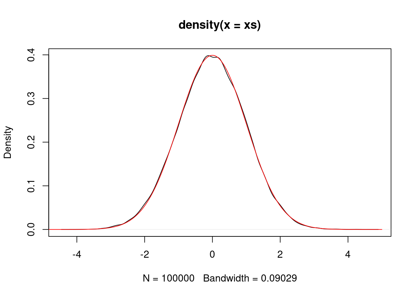
We can simulate an \({\rm Exponential}(1)\) random variable using a normal proposal.
P <- make.metropolis.hastings.kernel(dexp, make.normal.proposal(1.0))
xs <- simulate.chain(P, 1, 100000)
plot(density(xs))
vs <- seq(0,5,0.01)
lines(vs, dexp(vs), col="red")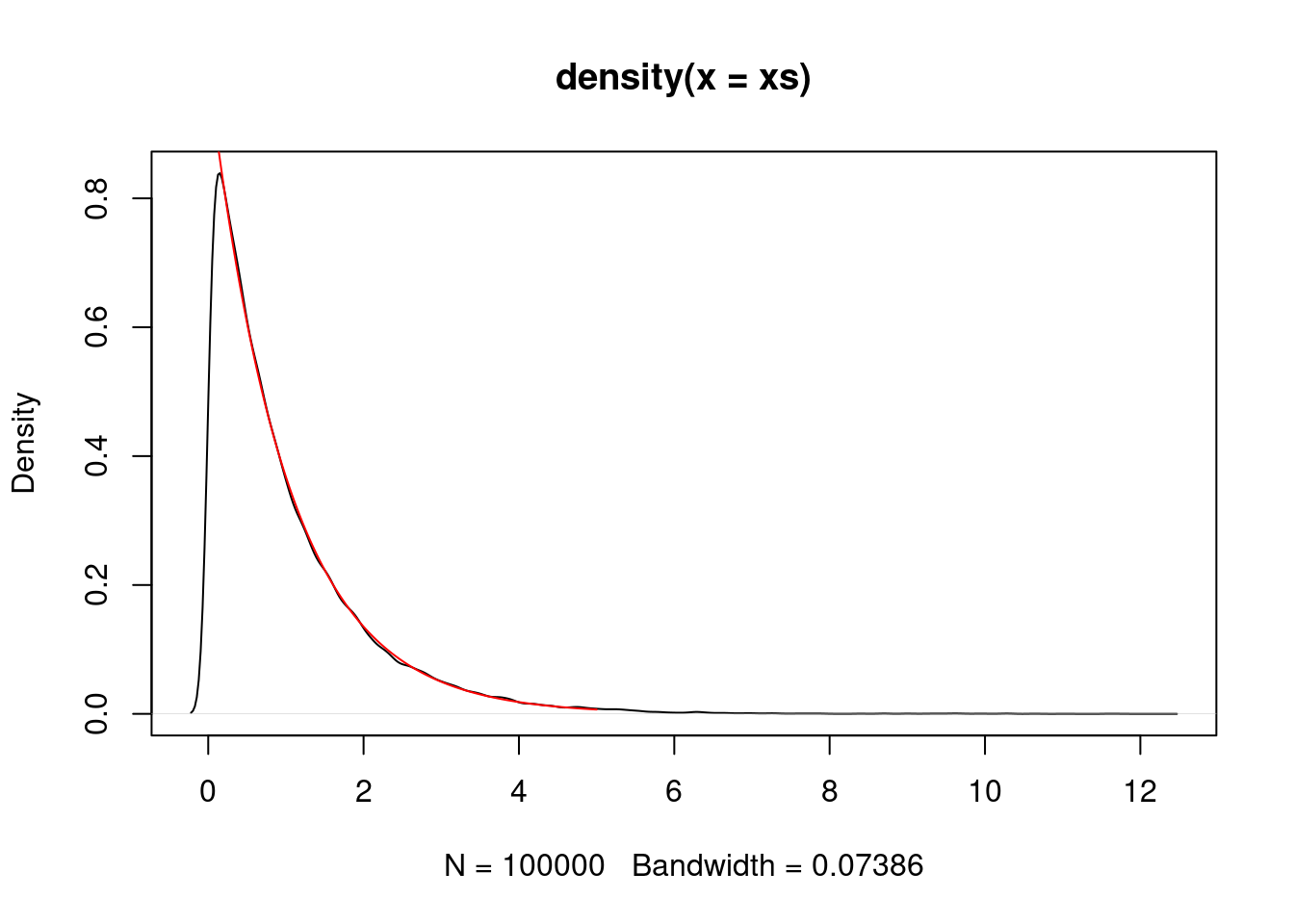
Actually, the proposal in the above two cases is “symmetric” in the sense that \(q(x,y) = q(y,x)\) for any \(x,y \in \mathbb{R}\). We can check that the algorithm still works when \(q(x,y) \neq q(y,x)\) and also show that it works for discrete random variables.
step.proposal <- list()
step.proposal$sample <- function(x) x + sample(c(-1,1), 1, prob = c(0.4,0.6))
step.proposal$density <- function(x,y) ifelse(y < x, 0.4, 0.6)

P <- make.metropolis.hastings.kernel(function(x) ifelse(x >= 1 && x <= 10, 1/x, 0), step.proposal)
xs <- simulate.chain(P, 1, 100000)
hist(xs, breaks=seq(min(xs)-0.5, max(xs)+0.5, 1), probability = TRUE, ylim=c(0,0.5))
vs <- seq(1,10,1)
points(vs, 1/vs/sum(1/vs), col="red", pch=20)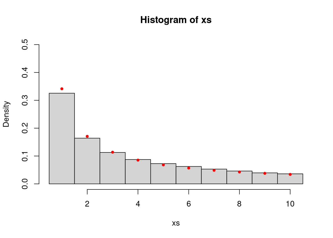
Finally, we can visualize how the chain depends on the choice of proposal standard deviation. In particular, this controls where the chain makes frequent moderate jumps, infrequent large jumps or very frequent but very small jumps. In practice, it is important to choose the proposal variance (or covariance in multivariate settings) to control the frequency and size of jumps.
P <- make.metropolis.hastings.kernel(dnorm, make.normal.proposal(1.0))
xs <- simulate.chain(P, 0, 1000)
plot(xs, pch=20)
P <- make.metropolis.hastings.kernel(dnorm, make.normal.proposal(10.0))
xs <- simulate.chain(P, 0, 1000)
plot(xs, pch=20)
P <- make.metropolis.hastings.kernel(dnorm, make.normal.proposal(0.1))
xs <- simulate.chain(P, 0, 1000)
plot(xs, pch=20)
Validity
In order to show that P leaves \(\pi\) invariant, we need to check \(\pi P=\pi\), i.e. \[\int_{\mathsf{X}}\pi({\rm d}x)P(x,A)=\pi(A),\qquad A\in\mathcal{X}.\]
Verifying \(\pi P = \pi\) is in fact extremely difficult in general, as is determining the invariant measure of a given Markov kernel. The \(\pi\)-invariance of the Metropolis–Hastings Markov chain is a special case of the \(\pi\)-invariance of \(\pi\)-reversible Markov chains.
Definition. A \(\pi\)-reversible Markov chain is a stationary Markov chain with invariant probability measure \(\pi\) satisfying \[\mathsf{P}_{\pi}(X_{0}\in A_{0},\ldots,X_{n}\in A_{n})=\mathsf{P}_{\pi}(X_{0}\in A_{n},\ldots,X_{n}\in A_{0}).\]
Fact. It suffices to check that for any \(A,B \in \mathcal{X}\), \[\mathsf{P}_{\pi}(X_{0}\in A,X_{1}\in B)=\mathsf{P}_{\pi}(X_{0}\in B,X_{1}\in A),\] i.e. \[\int_{A}\pi({\rm d}x)P(x,B)=\int_{B}\pi({\rm d}x)P(x,A).\]
Moreover, \(\pi\)-invariance is immediate by considering \(A=\mathsf{X}\): \[\int_{\mathsf{X}}\pi({\rm d}x)P(x,B)=\int_{B}\pi({\rm d}x)P(x,\mathsf{X})=\pi(B).\]
That \(\int_{A}\pi({\rm d}x)P(x,B)=\int_{B}\pi({\rm d}x)P(x,A)\) implies reversibility is slightly laborious in the general state space context. You can verify this for discrete \(\mathsf{X}\).
Theorem. Let \(P(x,A)=\int_{A}p(x,z)\lambda({\rm d}z)+r(x)\mathbf{1}_{A}(x)\). If the detailed balance condition \[\pi(x)p(x,z)=\pi(z)p(z,x),\quad x,z\in\mathsf{X}\] holds then \(P\) defines a \(\pi\)-reversible Markov chain.
Proof. We have \[\begin{align} \int_{A}\pi({\rm d}x)P(x,B) &= \int_{A}\pi(x)\left[\int_{B}p(x,z)\lambda({\rm d}z)+r(x)\mathbf{1}_{B}(x)\right]\lambda({\rm d}x) \\ &= \int_{B}\pi(z)\left[\int_{A}p(z,x)\lambda({\rm d}x)\right]\lambda({\rm d}z)+\int_{A\cap B}\pi(x)r(x)\lambda({\rm d}x) \\ &= \int_{B}\pi(z)\left[\int_{A}p(z,x)\lambda({\rm d}x)+r(z)\mathbf{1}_{A}(x)\right]\lambda({\rm d}z) \\ &= \int_{B}\pi({\rm d}x)P(x,A). \end{align}\]
The key utility of detailed balance is it need only be checked pointwise: no integrals necessary!
Corollary. Any Metropolis–Hastings Markov chain is \(\pi\)-reversible.
Proof. We have \[\begin{align} \pi(x)p_{{\rm MH}}(x,z) &= \pi(x)q(x,z)\left[1\wedge\frac{\pi(z)q(z,x)}{\pi(x)q(x,z)}\right] \\ &= \left[\pi(x)q(x,z)\wedge\pi(z)q(z,x)\right] \\ &= \pi(z)q(z,x)\left[\frac{\pi(x)q(x,z)}{\pi(z)q(z,x)}\wedge1\right] \\ &= \pi(z)p_{{\rm MH}}(z,x). \end{align}\]
Many Markov chains used in statistics are constructed using reversible Markov transition kernels.
If \(P_{{\rm MH}}\) is \(\pi\)-reversible and \(\pi\)-irreducible then it is positive and has \(\pi\) as its invariant probability measure. Verifying \(\pi\)-irreducibility is often very easy. For example, \(\pi(A)>0\), \(A\in\mathcal{X}\) and \(q(x,A)>0\), \(x\in\mathsf{X}\), \(A\in\mathcal{X}\).
Theorem [Tierney (1994, Corollary 2), Roberts & Rosenthal (2008, Theorem 8)]. Every \(\pi\)-irreducible, full-dimensional Metropolis–Hastings Markov chain is Harris recurrent.
Combining Markov kernels
We can easily construct \(\pi\)-invariant Markov chains out of different \(\pi\)-invariant Markov transition kernels. In practice, such hybrid chains are commonplace. For example, the Gibbs sampler.
Generally speaking, we will have \((P_{s})_ {s \in S}\) and we will try to make a mixture, cycle or combination of the two out of them.
Definition. A Markov kernel \(P\) is a mixture of the Markov kernels \((P_{s})_{s\in S}\) if \[P(x,A)=\sum_{s\in S}w(s)P_{s}(x,A),\] where \(w\) is a p.m.f. (independent of \(x\)). Alternatively, \(P=\sum_{s\in S}w(s)P_{s}\).
Fact. A mixture of \(\pi\)-invariant Markov kernels is \(\pi\)-invariant.
Proof. Let \(A \in \mathcal{X}\). Then \[\pi P(A)=\sum_{s\in S}w(s)\pi P_{s}(A)=\sum_{s\in S}w(s)\pi(A)=\pi(A). □\]
Definition. A Markov kernel \(P\) is a cycle of Markov kernels \(P_{1}\) and \(P_{2}\) if \[P(x,A)=\int_{\mathsf{X}}P_{1}(x,{\rm d}z)P_{2}(z,A),\] i.e., \(P=P_{1}P_{2}\).
Fact. A cycle of \(\pi\)-invariant Markov kernels is \(\pi\)-invariant.
Proof. Let \(A \in \mathcal{X}\). Then \[\pi P(A)=\pi P_{1}P_{2}(A)=\pi P_{2}(A)=\pi(A). □\]
That’s all you need to know to construct some sophisticated Markov chains!
If P is \(\pi\)-irreducible then so is a mixture including P with positive probability. The same is not necessarily true for cycles, but it is often true in practice.
A mixture of \(\pi\)-reversible Markov kernels is \(\pi\)-reversible. A cycle of \(\pi\)-reversible Markov kernels is generally not \(\pi\)-reversible.