Numerical Optimisation
An optimisation problem is the problem of finding the best solution from all feasible solutions. There are genenally speaking two types of optimisation problems: continuous or discrete, which refers to whether the variables are continuous or discrete. We will focus on continuous optimisation problems. Without any loss of generality, just as in R functions, we try to minimise (rather than maximise) a function.
The standard form of a continuous optimisation problem is as follows:
\[ \begin{eqnarray} \arg\min_x f(x) \ \mathrm{ subject \ to } \ & g_i(x)\le 0 \mathrm{\ for \ } i=1,\ldots,m, \\ & h_j(x) = 0 \mathrm{\ for \ } j=1,\ldots,p \end{eqnarray} \] where \(f:\mathbb{R}^N \to \mathbb{R}\) is the objective function and \(g_i\) and \(h_j\) are constraints.
We will mainly discuss optimisation without constraints here, although we note that the R function optim can deal with box constraints if we choose the L-BFGS-B algorithm. The most common R function to deal with constrained optimisation problem is constrOptim.
One-Dimensional Optimisation
We start with the one-dimensional case where we can graph the function easily.
f <- function(x) cos(x) + cos(2*x) + sin(3*x)
curve(f, from=0, to=2*pi)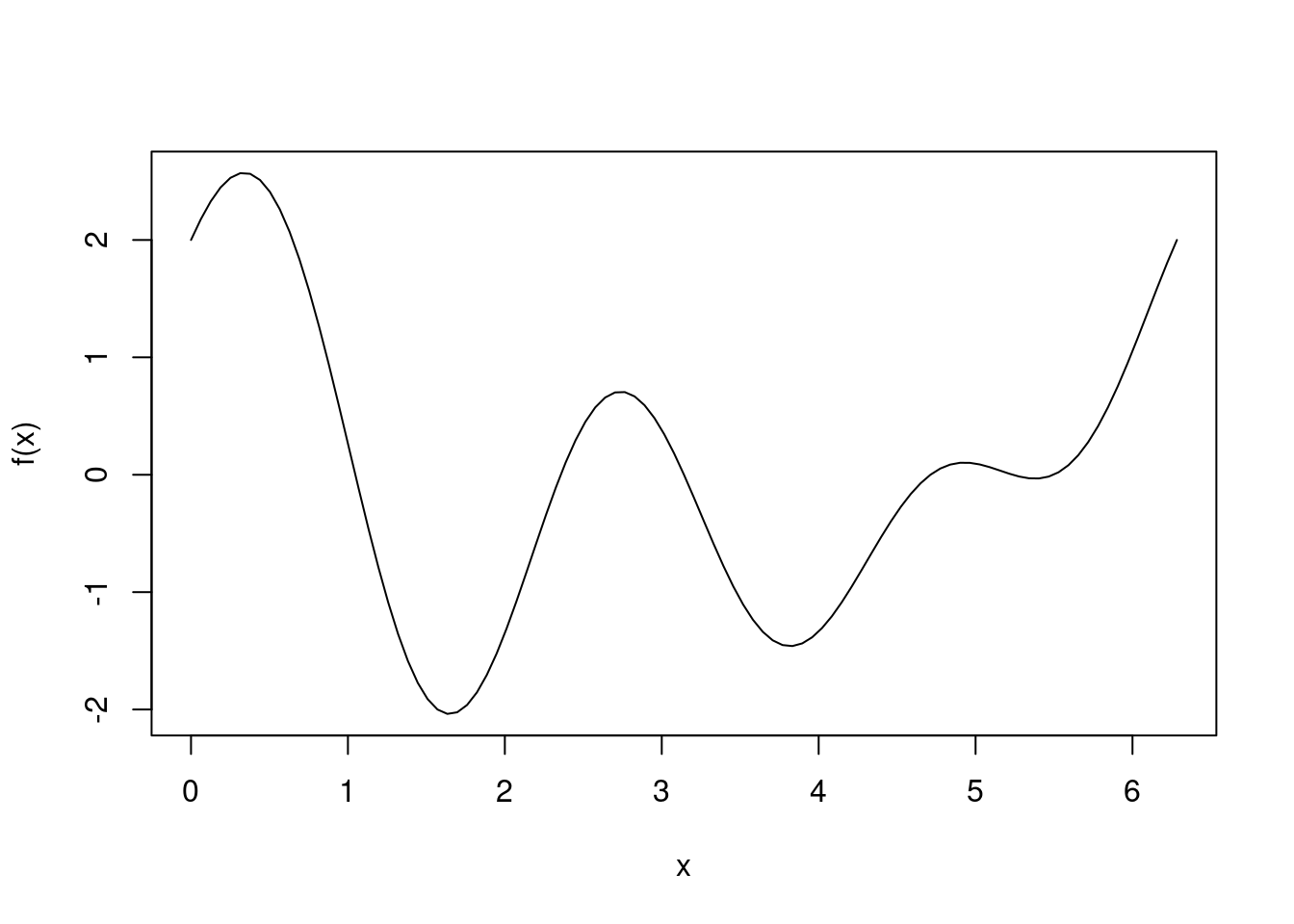
The optimize function
We apply the base R function optimize, which only works on functions of one variable, to this function:
optimize(f, interval=c(0, 2*pi))## $minimum
## [1] 3.817878
##
## $objective
## [1] -1.460318We see that the optimize function finds a local minimum at 3.82, but not the global minimum between 0 and \(2\pi\) at 1.65. If we change the search interval to \((0,1.5\pi)\), however, optimize does find the global minimum at 1.65, even though 3.82 is in \((0,1.5\pi)\).
optimize(f, interval=c(0, 1.5*pi))## $minimum
## [1] 1.648064
##
## $objective
## [1] -2.038528It seems using optimize is a hit or miss affair even with a simple function as above. What algorithm is behind this function? According to the documentation, the method is based on golden section search, which is known to work well for a uni-modal function where the minimum is within the search interval. If the search interval contains multiple extrema, the golden section search algorithm will converge to one of these extrema. But a plus is that no evaluation of derivatives is necessary.
We can also specify a paramter tol for optimize, which will stop the search once tolerance is reached.
optimize(f, interval=c(0,1.5*pi), tol=1e-2)## $minimum
## [1] 1.646619
##
## $objective
## [1] -2.038514Newton’s Method
Also known as the Newton-Raphson method, Newton’s method aims to find the root of a function \(g\). If we assume \(g\) has a Taylor expansion at \(x_0\), then \[ g(x) \approx g(x_0) + g'(x_0) (x-x_0). \] Setting this to 0 yields \[ 0 = g(x_0) + g'(x_0) (x-x_0) \\ -g(x_0) = g'(x_0) (x-x_0) \\ x = x_0 - \frac{g(x_0)}{g'(x_0)}. \] The idea of Newton is simply to iteratively apply the formula \[ x \leftarrow x - \frac{g(x)}{g'(x)}. \] There is a nice animation on wikipedia to show how Newton’s method works.
In order to apply it to the optimisation problem, we solve for \(f'(x)=0\).
f_sym <- expression(cos(x) + cos(2*x) + sin(3*x))
f1_sym <- D(f_sym, 'x'); f1 <- function(x) eval(f1_sym)
f2_sym <- D(f1_sym, 'x'); f2 <- function(x) eval(f2_sym)
x <- 2
for (i in 1:6) {
  x <- x - f1(x) / f2(x); cat(x, '\n')
}
## 1.371591
## 1.686732
## 1.647531
## 1.648062
## 1.648062
## 1.648062x <- 1
for (i in 1:6) {
x <- x - f1(x) / f2(x); cat(x, '\n')
}## -37.61615
## -37.2677
## -37.35961
## -37.3609
## -37.3609
## -37.3609As one can see, if the initial guess is somewhat close to a local minimum, then convergence to that minimum is rapid. But if the initial guess is not that close (which is hard to know beforehand), then the value Newton’s method converges to seems to be quite willful. Let’s see what the function is like near -37:
curve(f, from=-40, to=-30)
It seems -37.36 is a local maximum, which is not surprising since Newton’s method doesn’t distinguish between mimima and maxima. Another downside of Newton’s method is the requirement of second derivatives, which may not be available all the time.
One dimensional optimisation problems should be easy, but as we have seen, even these “easy” problems can be troublesome for algorithms if we simply apply them blindly.
Multi-dimensional Optimisation
Most optimisation problems we will encounter will be multi-dimensional. I will divide common optimisation algorithms into three categories:
- Simplex methods – only uses the value of the function
- Gradient type methods – uses the value of the function and its gradient vector
- Newton type methods – uses the value of the function, its gradient vector, and its Hessian matrix (or an approximation)
There are two main functions for multi-dimensional optimisation in R, nlm (non-linear minimisation), which uses a Newton-type algorithm, and optim, which has a choice of algorithms: Nelder-Mead, BFGS (Broyden, Fletcher, Goldfarb and Shanno), CG (conjugate gradient), L-BFGS-B (Byrd et al’s version of BFGS that is has low memory requirements and allows box constraints), SANN (simulated annealing), and Brent (use the one-dimensional optimize function discussed previously).
Simplex methods
Also known as the downhill simplex method, the Nelder-Mead algorithm is the most well-known simplex method. It is a direct search method based on comparing values of the function at various points. Its advantage is that it does not need to compute any derivatives. Its disadvantages are: the method is heuristic, it only converges to local minima, it may converge to non-stationary points, and it is reputed to be slow. The general idea is to start with a simplex (a polytope with \(n+1\) vertices in \(n\) dimensions, so a triangle in \(\mathbb{R}^2\)) then reflect, expand, contract, or shrink the simplex depending on values of the functions at vertices of this simplex.
Gradient type methods
The most well known gradient type method is the steepest descent (also known as gradient descent) algorithm. In order to minimise a differentiable multi-variable function \(f(x)\), \(x\in\mathbb{R}^n\), we iteratively take \[x \leftarrow x - \gamma \nabla f(x)\] where \(\gamma\) is small, i.e. we take a small step where the value of \(f\) is decreasing the fastest. We can choose \(\gamma\) by conducting a line-search to ensure the value of \(f\) is decreasing as fast as possible.
This relatively simple (both conceptually and in terms of ease of programming) method is known to relatively slow and can zigzag (if applied to e.g. the Rosenbrock function). Neither optim nor nlm uses the steepest descent algorithm.
A well-known improved gradient type method is the conjugate gradient (CG) algorithm. The main idea is that the search direction at each step should be conjugate toward search directions at previous step, so one avoids zigzag of classic steepest descent. In fact, if the function to be minimised is quadratic, then the conjugate gradient algorithm is guaranteed to reach the minimum in exactly \(n\) steps if the input to the function is \(n\)-dimensional (ignoring numerical errors). The conjugate gradient tend to perform better than the classical steepest descent even on general nonlinear functions, but not as well as Newton type methods.
Newton type methods
Recall that with Newton’s method for one-dimensional functions, we need the first two derivatives of the function we try to minimise. For multi-dimensional function, Newton’s method becomes \[x \leftarrow x - [Hf(x)]^{-1} \nabla f(x),\] where we need to compute the matrix inverse of the Hessian, which can be expensive for multi-dimensional problems since the Hessian matrix may be very large. Numerically computing the inverse of the Hessian matrix is in any case undesirable. Quasi-Newton methods aim to replace the inverse Hessian matrix by a reasonable estimate.
The most common quasi-Newton method is BFGS and its close relative L-BFGS. Details regarding the BFGS algorithm can be found on wikipedia, where \(B_k\) is an approximation to the Hessian matrix and its inverse is never computed. Rather, \(B_{k+1}^{-1}\) is computed using \(B_k^{-1}\), without performing an explicit matrix inversion.
The BFGS algorithm will store both \(B_k\) and \(B_k^{-1}\), which are likely to be dense matrices. This causes memory problems when the dimension is higher than say 1000. The low memory version of BFGS, L-BFGS, solves this problem by storing a few vectors (rather than the full approximate Hessian matrix and its inverse) that represents \(B_k\).
Simulated Annealing
Unlike the three types of techniques we have discussed so far, simulated annealing is supposed to be able to find the global minimum of a function. But it is slow and often fails to find the global minimum in any case. On the plus side, it only uses the value of the fuction, just like the simplex method. The implementation in optim uses a Metropolis function for the acceptance probability.
Generally speaking, Newton type methods perform better than gradient type methods, but conjugate gradient falls somewhere between steepest descent and Newton type methods. If it were easy for simulated annealing to find the global minimum of a function, there would be no need for any other optimisation techniques. The fact that there are a plethora of optimisation algorithms says at least something about the efficacy of simulated annealing.
Nonlinear least squares problems
Assume we have a dataset \((x_1,y_1),(x_2,y_2), \ldots, (x_m,y_m)\) and a model \(y=f(x,\beta)\) where \(\beta=(\beta_1,\beta_2,\ldots,\beta_n)\) are parameters of the model \(f\). We define residuals to be \[r_i(\beta) = y_i - f(x_i,\beta).\] In a nonlinear least squares problem, we aim to find \(\beta\) such that the sum of squares of residuals is minimised: \[\arg\min_\beta \sum_{i=1}^m r_i^2 = \arg\min_\beta \sum_{i=1}^m (y_i - f(x_i,\beta))^2.\] A subclass of optimisation algorithms work just for nonlinear least squares problems. We briefly discuss the two most famous examples: the Gauss-Newton algorithm and the Levenberg-Marquardt algorithm.
The Gauss-Newton algorithm is a closely related to Newton’s method for general optimisation problems. The difference (improvement) is that the Gauss-newton algorithm approximates the Hessian matrix of the objective function \(\sum_{i=1}^m (y_i - f(x_i,\beta))^2\) using Jacobian matrix \(J_r\) of the residue function, i.e. it pretends the Hessian matrix is \(2J_t^t J_r\), which may or may not be invertible: \[ \beta \leftarrow \beta - (J_r^t J_r)^{-1} J_r^t r(\beta).\] This works well in practice but is not guaranteed to converge (at least theoretically).
The Levenberg-Marquardt algorithm address this problem by damping. It pretends the Hessian matrix is \(2(J_r^t J_r + \lambda I)\), where \(\lambda\) is a small damping parameter and \(I\) is the identity matrix: \[\beta \leftarrow \beta - (J_r^t J_r + \lambda I)^{-1} J_r^t r(\beta).\] We note that if \(\lambda=0\) then we obtain the Gauss-Newton algorithm. But if \(\lambda\) is large, then we obtain the steepest descent algorithm. Therefore we would like to use a \(\lambda\) that is as small as possible but does not cause numerical stability issues. A useful strategy is to reduce \(\lambda\) at every iteration as long as the squared residue is decreased, but increasing \(\lambda\) sufficiently to ensure the squared residue does not increase. The matrix \(J_r^t J_r + \lambda I\) is guaranteed to be invertible for at least some \(\lambda\).
Stochastic Gradient Descent
Methods such as BFGS and Levenberg-Marquardt are highly efficient but they compute the gradient vectors taking into account all of the dataset. Such methods are known as batch methods. In many big data applications, however, the dataset can be too large to hold in computer memory at the same time. This is the main motivation behind stochastic gradient descent (SGD), which changes the parameter in the negative gradient direction taking into account only a few data samples. SGD is especially popular for the training of neural networks, where the full back propagation over the full training set can be very expensive computationally.
In the simplest form, SGD takes on the following form: \[\beta \leftarrow \beta - \gamma r_i \nabla r_i(\beta),\] where \(i\) cycles through all data points in a deterministic or random fashion. One can also combine a number of data samples into “mini-batches” and update the parameter \(\beta\) using samples in each minibatch.