Advantages

• Code and documentation are consistent with each other, since they are produced from the same source.
• One can focus on readability of the output document.
• One can emphasize thought processes behind the code more clearly.

How to use RMarkdown

If you already are familiar with a flavor of Markdown, RMarkdown primarily extends this with the ability to write and call R code.

This Markdown cheat sheet is pretty self-explanatory. One can include R code chunks by inserting lines such as the following in an RMarkdown file.

```{r[, <any chunk options>]}
# R code
```

For example, writing

```{r}
1 + 2
```

gives rise to

1 + 2

## [1] 3

in the rendered document. Many of the webpages for this website are written using R Markdown, so you can view their source to see further examples. In RStudio, documents are rendered by clicking the “Knit” button.

The first few lessons provided by RStudio may be helpful. There is an RMarkdown cheat sheet as well.

Application to data science

In many data science workflows, one uses a variety of functions to load and clean data, analyze it, and then display outputs and visualizations. A literate programming approach to these high-level tasks makes them more transparent and reproducible. Furthermore, the document can be designed with the intended audience in mind.

Example

This example concerns historical exchange rate data against the Euro, obtained from the European Central Bank.

This page is written in RMarkdown: you can view the source by clicking the “View source” link at the bottom of the page.

eurofxref <- read.csv("../../static/data/eurofxref-hist.csv", na.strings="N/A")
eurofxref$Date <- as.Date(eurofxref$Date)
n <- length(eurofxref$Date)

We can plot the USD and GBP rates over time.

ylim <- range(c(eurofxref$USD, eurofxref$GBP))
plot(eurofxref$Date, eurofxref$USD, pch=20, ylim=ylim,
  main="Daily exchange rate for USD (black) and GBP (red) against the Euro",
  xlab="Date", ylab="Price of 1 Euro")
points(eurofxref$Date, eurofxref$GBP, pch=20, col="red")

We consider the daily change in exchange rates for both currencies.

diff.USD <- diff(eurofxref$USD)
diff.GBP <- diff(eurofxref$GBP)
plot(eurofxref$Date[1:(n-1)], diff.USD, pch=20,
  main="Daily difference in exchange rate for USD (black) and GBP (red)
    against the Euro", xlab="Date", ylab="Difference in price of 1 Euro")
points(eurofxref$Date[1:(n-1)], diff.GBP, pch=20, col="red")

The differences may be independent normal random variables. We can plot kernel density estimates for rescaled differences and an appropriate normal density to check this.

rescaled.diff.USD <- diff.USD/sd(diff.USD)
rescaled.diff.GBP <- diff.GBP/sd(diff.GBP)

vs <- seq(-10,10,0.01)
plot(density(rescaled.diff.USD), main="Kernel density estimates for USD (black)
  and GBP (red), with standard normal density (blue)")
lines(density(rescaled.diff.GBP), col="red")
lines(vs, dnorm(vs), col="blue")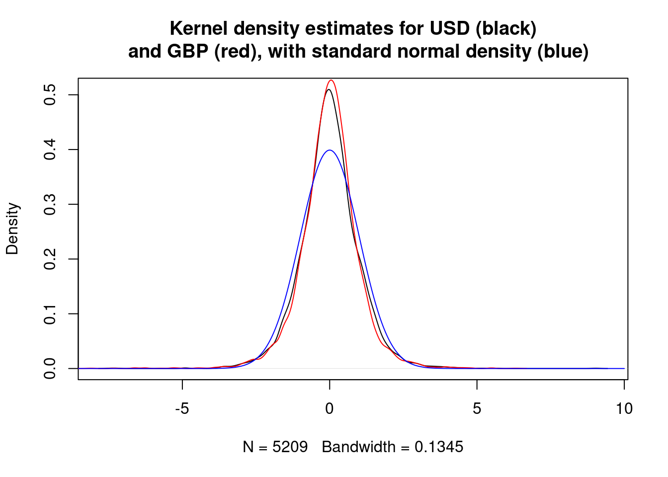

The estimated densities for the rescaled differences appear to be similar to each other, but different from a standard normal.

We can perform a Shapiro–Wilk test for each of the rescaled differences to see if they could be normal.

# shapiro.test sample size must be between 3 and 5000
shapiro.test(rescaled.diff.USD[1:5000])

## 
## 	Shapiro-Wilk normality test
## 
## data:  rescaled.diff.USD[1:5000]
## W = 0.97014, p-value < 2.2e-16

shapiro.test(rescaled.diff.GBP[1:5000])

## 
## 	Shapiro-Wilk normality test
## 
## data:  rescaled.diff.GBP[1:5000]
## W = 0.93928, p-value < 2.2e-16

There is very strong evidence against the rescaled differences being normally distributed.

We can also perform a Kolmogorov–Smirnov test to see if the rescaled differences could be from the same distribution.

ks.test(rescaled.diff.USD, rescaled.diff.GBP)

## Warning in ks.test.default(rescaled.diff.USD, rescaled.diff.GBP): p-value will
## be approximate in the presence of ties

## 
## 	Asymptotic two-sample Kolmogorov-Smirnov test
## 
## data:  rescaled.diff.USD and rescaled.diff.GBP
## D = 0.024573, p-value = 0.0861
## alternative hypothesis: two-sided

The p-value is not that small, so evidence against the two rescaled differences coming from the same distribution is weak.

When not to use RMarkdown

As suggested above, literate programming is very good for presenting a high-level data analysis. It is often used to communicate how data is processed and how conclusions are drawn.

It is not common to write packages of low-level functionality entirely using RMarkdown. Instead, people typically write R scripts with helpful comments that are easy to understand, and use function and variable names that ease understanding of the code itself. It is possible to use special “roxygen” comments that can automatically be turned into help documentation for users of those functions: we will cover this in more detail later.

An RMarkdown file has Markdown text and specially delimited code chunks, which can be processed to produce the desired output. An alternative is to write an R script with specially delimited Markdown chunks. These chunks are automatically ignored by R as they are parsed as comments, but can optionally be converted into a literate programming document by the knitr::spin function.