5. Data reshaping with dplyr and tidyr

This section is the natural continuation of the previous one, which focussed on data transformation with dplyr. Here we show how to use the tidyr package, which provides tools for reshaping your data for the purpose of modelling and visualization, and we will illustrate more features of dplyr. As for the previous sections, here we cover the basics and we refer to the relevant chapter of “R for Data Science” for more details.

Pivoting your data

To illustrate the reshaping tools provided by tidyr, here we look at another electricity demand data set. In particular, we consider an Irish smart meter data set which can be found in the electBook package. At the time of writing electBook is available only on Github, hence we need to install it from there using devtools:

library(magrittr)
library(tidyr)
library(dplyr)
library(ggplot2)

# Install electBook only if it is not already installed
if( !require(electBook) ){
  library(devtools)
  install_github("mfasiolo/electBook")
  library(electBook)
}

## TTR          (NA -> 0.24.4    ) [CRAN]
## xts          (NA -> 0.13.2    ) [CRAN]
## quantmod     (NA -> 0.4.26    ) [CRAN]
## zoo          (NA -> 1.8-12    ) [CRAN]
## quadprog     (NA -> 1.5-8     ) [CRAN]
## RcppArmad... (NA -> 0.12.8.0.0) [CRAN]
## urca         (NA -> 1.3-3     ) [CRAN]
## tseries      (NA -> 0.10-55   ) [CRAN]
## timeDate     (NA -> 4032.109  ) [CRAN]
## lmtest       (NA -> 0.9-40    ) [CRAN]
## fracdiff     (NA -> 1.5-3     ) [CRAN]
## forecast     (NA -> 8.21.1    ) [CRAN]
## ── R CMD build ─────────────────────────────────────────────────────────────────
## * checking for file ‘/tmp/RtmpF7xGYf/remotesd32c335ccafd/mfasiolo-electBook-38d7020/DESCRIPTION’ ... OK
## * preparing ‘electBook’:
## * checking DESCRIPTION meta-information ... OK
## * checking for LF line-endings in source and make files and shell scripts
## * checking for empty or unneeded directories
## * building ‘electBook_0.0.1.tar.gz’

Then we load the smart meter data:

data(Irish)

Irish is a list, where Irish$indCons is a data.frame containing electricity demand data over one year, at 30min resolution, for more than 2000 smart meters. We store it as a separate object:

indCons <- Irish$indCons
dim(indCons)

## [1] 16799  2672

head(indCons[ , 1:10])

##      I1002 I1003 I1004 I1005 I1013 I1015 I1018 I1020 I1022 I1024
## 8114 0.022 0.593 2.002 0.755 0.035 0.398 0.547 0.376 0.229 1.030
## 8115 0.133 0.707 1.602 0.898 0.112 0.689 0.603 0.275 0.198 0.807
## 8116 0.094 0.684 1.525 0.736 0.046 0.407 0.511 0.259 0.201 0.859
## 8117 0.023 0.563 1.393 0.738 0.036 0.223 0.593 0.249 0.212 0.210
## 8118 0.133 0.489 1.221 0.849 0.065 0.132 0.570 0.241 0.121 0.056
## 8119 0.090 0.521 1.032 0.695 0.093 0.117 0.481 0.122 0.127 0.169

Each column contains the demand of a different customer. In order to limit the computational burden, below we focus on a subset of 100 customers:

indCons <- indCons[ , 1:100]

Now, suppose that we want to plot the consumption of some of the customers over time, on the same plot. Using base R, one way of doing this is:

matplot(indCons[1:(48*7), 1:3], type = 'l')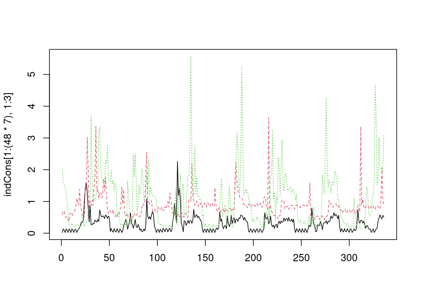

Here we are plotting the consumption of the first three customers over the first 7 days (we have 48 observations per day). To do the same in ggplot2 we need to put the data in a “long” format, that is we need a data.frame where one column contains the demand values and another indicates to which customer each demand value belongs to. This can be achieved easily using tidyr::pivot_longer:

longDat <- indCons %>% pivot_longer(cols = everything(), names_to = "ID", values_to = "dem") %>% dplyr::arrange(ID)
head(longDat, 5)

## # A tibble: 5 × 2
##   ID      dem
##   <chr> <dbl>
## 1 I1002 0.022
## 2 I1002 0.133
## 3 I1002 0.094
## 4 I1002 0.023
## 5 I1002 0.133

tail(longDat, 5)

## # A tibble: 5 × 2
##   ID      dem
##   <chr> <dbl>
## 1 I1241 0.166
## 2 I1241 0.278
## 3 I1241 0.103
## 4 I1241 0.116
## 5 I1241 0.073

As you can see, the demand of all the customers has been aligned in a single vector, and the customer ID is reported in a separate column. In the call to pivot_longer, the cols argument specifies the set of columns whose names are values. The names_to argument specifies the name we wish to give to the variable whose values formed the column names in the original data set (the customer IDs). The values_to argument specifies the name we wish to give to the variable whose values were spread over the columns of the original data set (the electricity consumption).

One issue with the long format is that it uses more memory, in fact:

indCons %>% object.size %>% format(units = "MB")

## [1] "12.9 Mb"

longDat %>% object.size %>% format(units = "MB")

## [1] "25.6 Mb"

This is mainly due to the ID column, which pretty much doubles the memory needed to store our data. The problem can be alleviated by converting the ID variable from a character string to a factor:

longDat %<>% mutate(ID = as.factor(ID))
longDat %>% object.size %>% format(units = "MB")

## [1] "19.2 Mb"

The memory saving occurs because we store only one copy of the factor levels (which are character strings). This can be done directly in the call to pivot_longer, by specifying that the names must be transformed into a factor:

longDat <- indCons %>% pivot_longer(cols = everything(), names_to = "ID", values_to = "dem", names_transform = list(ID = as.factor)) %>% dplyr::arrange(ID)
longDat %>% object.size %>% format(units = "MB")

## [1] "19.2 Mb"

Having put the data in this format, we can try to plot the demand using ggplot2:

longDat %>% filter(ID %in% levels(ID)[1:3]) %>%
            group_by(ID) %>%
            slice(1:(48 * 7)) %>%
            ggplot(aes(x = 1:nrow(.), y = dem, col = ID)) +
            geom_line()

Here we are using filter to select the first three customers, then we group the data by customer ID and we use slice to select the first $48 \times 7$ observations for each customers. However, we didn’t quite get the plot we wanted, because the consumption of the three customers does not overlap, but it’s plotted sequentially along the $x$-axis. To get the ggplot2 equivalent of the plot we got with matplot, we need a variable going from 1 to $48 \times 7$ repeatedly for each of the customers. This is achieved as follows:

longDat %>% filter(ID %in% levels(ID)[1:3]) %>%
            group_by(ID) %>%
            slice(1:(48 * 7)) %>%
            mutate(counter = row_number()) %>%
            ggplot(aes(x = counter, y = dem, col = ID)) +
            geom_line()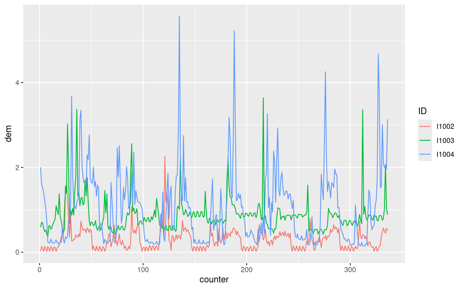

Where we used row_number within mutate to add a new counter variable to the data. counter is shown by the following plot:

longDat %>% filter(ID %in% levels(ID)[1:3]) %>%
            group_by(ID) %>%
            slice(1:(48 * 7)) %>%
            mutate(counter = row_number()) %>%
            ggplot(aes(x = 1:nrow(.), y = counter, col = ID)) +
            geom_line()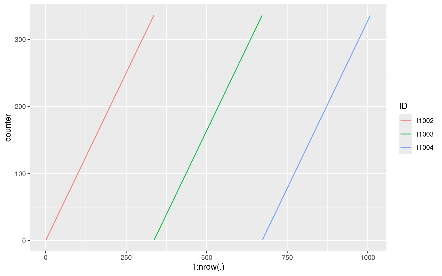

At this point you might (legitimately!) be wondering whether we would have been better off just sticking to matplot, which was much easier to use in this case. However, notice that once we got our data.frame in the long shape, we can use all the plot types and layers provided by ggplot2. In addition, we can use dplyr and ggplot2 to do more complicated things like:

longDat %>% group_by(ID) %>%
            slice(1:(48 * 7)) %>%
            mutate(counter = row_number()) %>%
            group_by(counter) %>%
            summarise(dem = sum(dem)) %>%
            ggplot(aes(x = 1:nrow(.), y = dem)) +
            geom_smooth() +
            geom_point()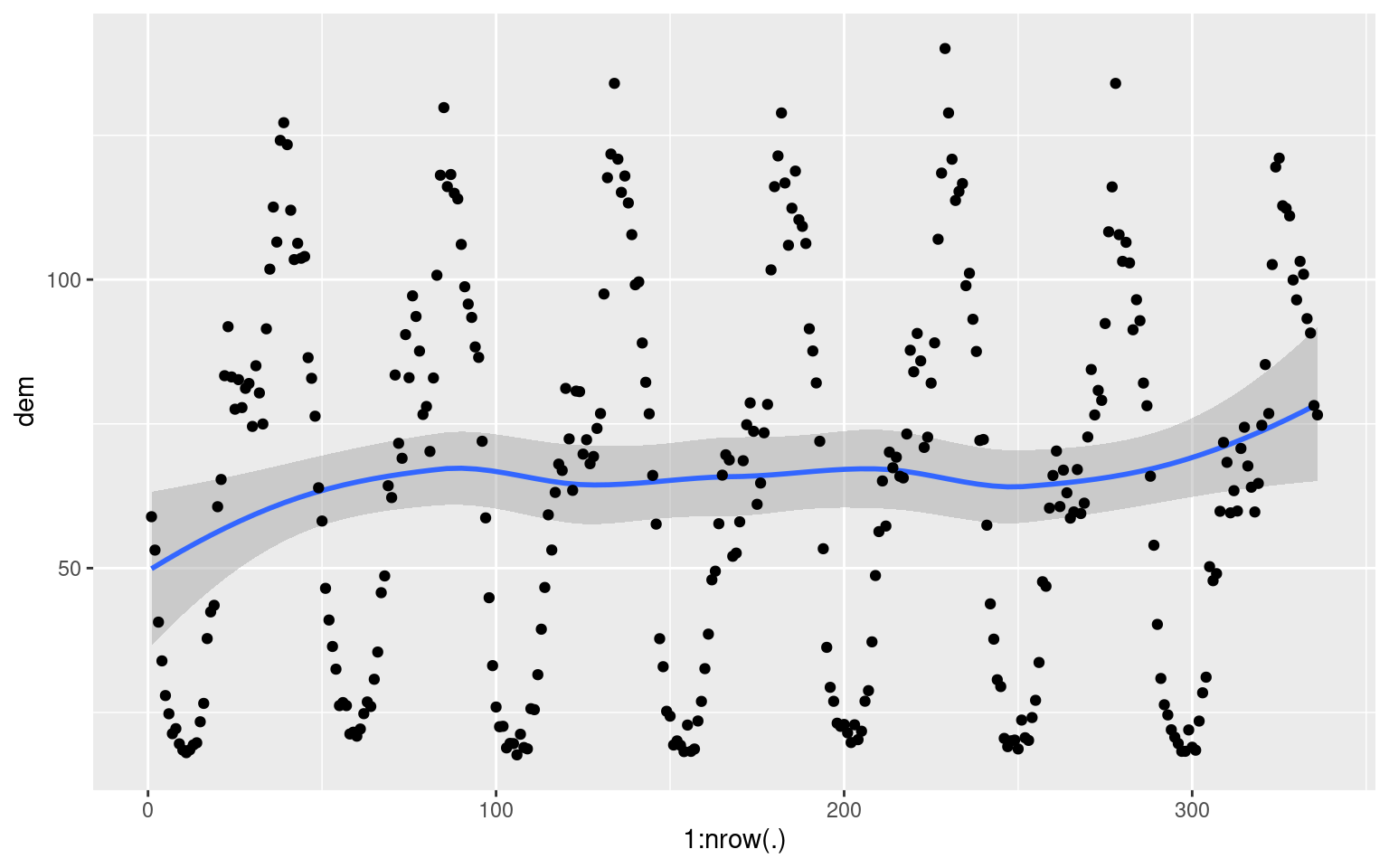

As an exercises, try to work out what the above code does, and what is being plotted.

For the purpose of illustration, let us add the counter variable to the whole longDat data set:

longDat %<>% group_by(ID) %>%
             mutate(counter = row_number()) %>%
             ungroup()

where we use ungroup to remove the grouping created by group_by. Now, suppose that we were given longDat, and that we wanted to spread it out on a wide format (as in the original indCons data set). We can achieve this using the tidyr::pivot_wider function:

wideDat <- longDat %>% pivot_wider(names_from = "ID", values_from = "dem")

print(wideDat, n = 5, width = 60, max_extra_cols = 0)

## # A tibble: 16,799 × 101
##   counter I1002 I1003 I1004 I1005 I1013 I1015 I1018 I1020
##     <int> <dbl> <dbl> <dbl> <dbl> <dbl> <dbl> <dbl> <dbl>
## 1       1 0.022 0.593  2.00 0.755 0.035 0.398 0.547 0.376
## 2       2 0.133 0.707  1.60 0.898 0.112 0.689 0.603 0.275
## 3       3 0.094 0.684  1.52 0.736 0.046 0.407 0.511 0.259
## 4       4 0.023 0.563  1.39 0.738 0.036 0.223 0.593 0.249
## 5       5 0.133 0.489  1.22 0.849 0.065 0.132 0.57  0.241
## # ℹ 16,794 more rows

As you can see we got back a wide data.frame, where the values of longDat$ID are variable names. Now, suppose that we wanted to transform wideDat back to a long format. Simply doing the following is not a good idea:

longDat2 <- wideDat %>% pivot_longer(cols = everything(), names_to = "ID", values_to = "dem", names_transform = list(ID = as.factor)) %>% dplyr::arrange(ID)
head(longDat2)

## # A tibble: 6 × 2
##   ID        dem
##   <fct>   <dbl>
## 1 counter     1
## 2 counter     2
## 3 counter     3
## 4 counter     4
## 5 counter     5
## 6 counter     6

tail(longDat2)

## # A tibble: 6 × 2
##   ID      dem
##   <fct> <dbl>
## 1 I1241 0.354
## 2 I1241 0.166
## 3 I1241 0.278
## 4 I1241 0.103
## 5 I1241 0.116
## 6 I1241 0.073

because the variable counter is considered to be an ID! The solution is specifying which columns we want to gather when reshaping the data:

longDat2 <- wideDat %>% pivot_longer(cols = I1002:I1241, names_to = "ID", values_to = "dem", names_transform = list(ID = as.factor)) %>% dplyr::arrange(ID)
head(longDat2)

## # A tibble: 6 × 3
##   counter ID      dem
##     <int> <fct> <dbl>
## 1       1 I1002 0.022
## 2       2 I1002 0.133
## 3       3 I1002 0.094
## 4       4 I1002 0.023
## 5       5 I1002 0.133
## 6       6 I1002 0.09

where we are using I1002:I1241 to specify that we want to gather all the columns included between I1002 and I1241. This worked well, but it required us to know the names of the two “limit” columns (I1002 and I1241) and there is the assumption that all the columns to be gathered are included between them (which is not always the case). A better alternative is the following:

longDat3 <- wideDat %>% pivot_longer(cols = starts_with("I1"), names_to = "ID", values_to = "dem", names_transform = list(ID = as.factor)) %>% dplyr::arrange(ID)

where we are using starts_with to gather all the columns that start with the “I1” string. The result is identical:

identical(longDat2, longDat3)

## [1] TRUE

As an exercise, you might want to think about what the following code does:

strange <- wideDat %>% pivot_longer(cols = c(I1002, I1003), names_to = "ID", values_to = "dem", names_transform = list(ID = as.factor))
strange

## # A tibble: 33,598 × 101
##    counter I1004 I1005 I1013 I1015 I1018 I1020 I1022 I1024 I1027 I1033 I1036
##      <int> <dbl> <dbl> <dbl> <dbl> <dbl> <dbl> <dbl> <dbl> <dbl> <dbl> <dbl>
##  1       1  2.00 0.755 0.035 0.398 0.547 0.376 0.229 1.03  0.07  0.79  0.602
##  2       1  2.00 0.755 0.035 0.398 0.547 0.376 0.229 1.03  0.07  0.79  0.602
##  3       2  1.60 0.898 0.112 0.689 0.603 0.275 0.198 0.807 0.041 0.361 0.565
##  4       2  1.60 0.898 0.112 0.689 0.603 0.275 0.198 0.807 0.041 0.361 0.565
##  5       3  1.52 0.736 0.046 0.407 0.511 0.259 0.201 0.859 0.027 0.363 0.527
##  6       3  1.52 0.736 0.046 0.407 0.511 0.259 0.201 0.859 0.027 0.363 0.527
##  7       4  1.39 0.738 0.036 0.223 0.593 0.249 0.212 0.21  0.047 0.215 0.609
##  8       4  1.39 0.738 0.036 0.223 0.593 0.249 0.212 0.21  0.047 0.215 0.609
##  9       5  1.22 0.849 0.065 0.132 0.57  0.241 0.121 0.056 0.019 0.133 0.203
## 10       5  1.22 0.849 0.065 0.132 0.57  0.241 0.121 0.056 0.019 0.133 0.203
## # ℹ 33,588 more rows
## # ℹ 89 more variables: I1039 <dbl>, I1041 <dbl>, I1042 <dbl>, I1044 <dbl>,
## #   I1047 <dbl>, I1052 <dbl>, I1054 <dbl>, I1055 <dbl>, I1057 <dbl>,
## #   I1058 <dbl>, I1059 <dbl>, I1060 <dbl>, I1061 <dbl>, I1062 <dbl>,
## #   I1064 <dbl>, I1065 <dbl>, I1067 <dbl>, I1069 <dbl>, I1073 <dbl>,
## #   I1075 <dbl>, I1076 <dbl>, I1077 <dbl>, I1079 <dbl>, I1081 <dbl>,
## #   I1082 <dbl>, I1083 <dbl>, I1086 <dbl>, I1091 <dbl>, I1093 <dbl>, …

Is the strange dataframe likely to be useful in practice?

Merging dataframes using joins

So far we only looked at Irish$indCons, which contains the individual electricity demand data. However, Irish contains also information about each customer:

survey <- as_tibble( Irish$survey )
head(survey)

## # A tibble: 6 × 12
##   ID    meanDem SOCIALCLASS OWNERSHIP BUILT.YEAR HEAT.HOME HEAT.WATER
##   <chr>   <dbl> <fct>       <chr>          <dbl> <chr>     <chr>     
## 1 I1002   0.208 DE          O               1975 Other     Elec      
## 2 I1003   0.622 C1          O               2004 Other     Other     
## 3 I1004   0.962 C1          O               1987 Other     Elec      
## 4 I1005   0.640 C1          O               1930 Other     Other     
## 5 I1013   0.241 C2          O               2003 Other     Elec      
## 6 I1015   0.463 DE          R               1989 Elec      Other     
## # ℹ 5 more variables: WINDOWS.doubleglazed <chr>,
## #   HOME.APPLIANCE..White.goods. <dbl>, Code <int>, ResTariffallocation <fct>,
## #   ResStimulusallocation <fct>

Here we have, among others, the built year of the building, the type of heating and the number of appliances (see ?Irish for more details). We also have some extra information in the following slot:

extra <- as_tibble( Irish$extra )
head(extra)

## # A tibble: 6 × 7
##    time   toy dow   holy    tod  temp dateTime           
##   <int> <dbl> <fct> <lgl> <dbl> <dbl> <dttm>             
## 1     1 0.986 Wed   FALSE     0     4 2009-12-29 23:00:00
## 2     2 0.986 Wed   FALSE     1     4 2009-12-29 23:30:00
## 3     3 0.986 Wed   FALSE     2     4 2009-12-30 00:00:00
## 4     4 0.986 Wed   FALSE     3     4 2009-12-30 00:30:00
## 5     5 0.986 Wed   FALSE     4     4 2009-12-30 01:00:00
## 6     6 0.986 Wed   FALSE     5     4 2009-12-30 01:30:00

In particular, we have some standard variables indicating the time of year, temperature and time of day (see ?Irish).

Now, for the purpose of modelling and of producing ggplot2-based visualizations, it makes sense to try to merge the dataframes on individual consumption (indCons), household information (survey) and other variables (extra) in a single dataframe. Joining indCons with extra is quite simple:

allDat <- longDat %>% cbind(extra) #left_join(extra, by = NULL)
head(allDat)

##      ID   dem counter time       toy dow  holy tod temp            dateTime
## 1 I1002 0.022       1    1 0.9863014 Wed FALSE   0    4 2009-12-29 23:00:00
## 2 I1002 0.133       2    2 0.9863014 Wed FALSE   1    4 2009-12-29 23:30:00
## 3 I1002 0.094       3    3 0.9863014 Wed FALSE   2    4 2009-12-30 00:00:00
## 4 I1002 0.023       4    4 0.9863014 Wed FALSE   3    4 2009-12-30 00:30:00
## 5 I1002 0.133       5    5 0.9863014 Wed FALSE   4    4 2009-12-30 01:00:00
## 6 I1002 0.090       6    6 0.9863014 Wed FALSE   5    4 2009-12-30 01:30:00

in fact cbind will bind the columns of longDat with 100 copies of extra (one copy for each customer). Hence now we can, for instance, look at the consumption of the first 3 customers as a function of the time of day tod, while distiguishing between working days and weekends:

allDat %>% filter(ID %in% levels(ID)[c(5, 10, 15)]) %>%
           mutate(weekend = dow %in% c("Sat", "Sun")) %>%
           ggplot(aes(x = tod, y = dem, group = ID, color = ID)) +
           geom_smooth() +
           facet_wrap(~ weekend)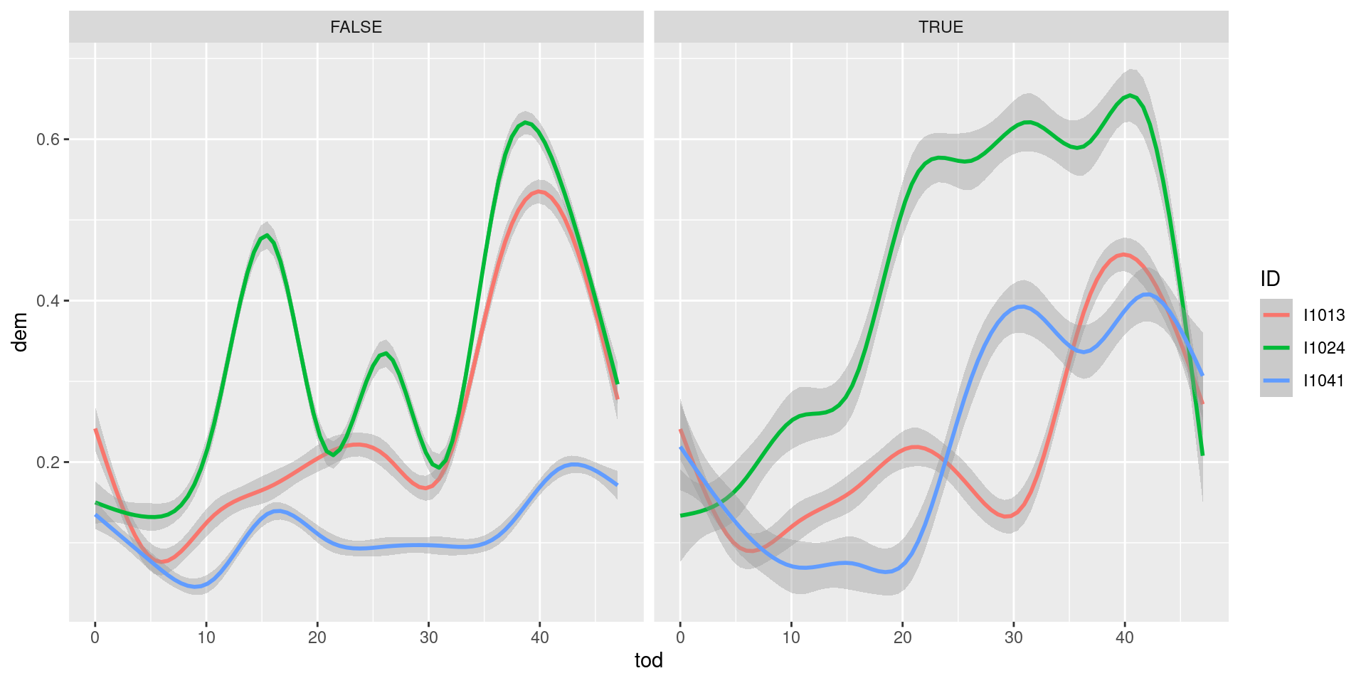

As you can see, customer I1024 is probably at home during afternoon weekends, hence his consumption is higher than during working days.

Now, how to add also the information in survey to allDat? The way to do it is:

allDat %<>% left_join(survey, by = "ID") %>%
            as_tibble()
head(allDat)

## # A tibble: 6 × 21
##   ID      dem counter  time   toy dow   holy    tod  temp dateTime           
##   <chr> <dbl>   <int> <int> <dbl> <fct> <lgl> <dbl> <dbl> <dttm>             
## 1 I1002 0.022       1     1 0.986 Wed   FALSE     0     4 2009-12-29 23:00:00
## 2 I1002 0.133       2     2 0.986 Wed   FALSE     1     4 2009-12-29 23:30:00
## 3 I1002 0.094       3     3 0.986 Wed   FALSE     2     4 2009-12-30 00:00:00
## 4 I1002 0.023       4     4 0.986 Wed   FALSE     3     4 2009-12-30 00:30:00
## 5 I1002 0.133       5     5 0.986 Wed   FALSE     4     4 2009-12-30 01:00:00
## 6 I1002 0.09        6     6 0.986 Wed   FALSE     5     4 2009-12-30 01:30:00
## # ℹ 11 more variables: meanDem <dbl>, SOCIALCLASS <fct>, OWNERSHIP <chr>,
## #   BUILT.YEAR <dbl>, HEAT.HOME <chr>, HEAT.WATER <chr>,
## #   WINDOWS.doubleglazed <chr>, HOME.APPLIANCE..White.goods. <dbl>, Code <int>,
## #   ResTariffallocation <fct>, ResStimulusallocation <fct>

where we used left_join to do the merging and as_tibble to convert the data.frame to a tibble (simply because it prints out more nicely). In left_join we set by = "ID", because ID is the common variable that we use to the matching between the demand data in allDat and the household information data in survey. In this case ID is said to be a primary key of the survey dataframe because it uniquely identifies each of its rows. It is also a foreign key because it allows to associate each row of allDat to one of the rows of survey. Having added the survey information, we can, for example, check how the distribution of the total per-customer yearly consumption changes with the number of appliances:

allDat %>% group_by(ID) %>%
   summarise(dem = sum(dem),
             appli = first(HOME.APPLIANCE..White.goods.)) %>%
   ggplot(aes(x = dem, group = appli, colour = appli)) +
   geom_density()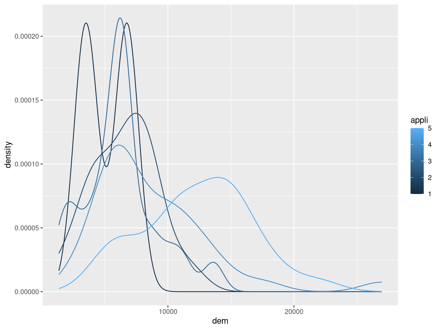

Hence, it seems that the (total, per customer) consumption increases with the number of white goods (this becomes clearer if you consider the whole data set rather than a subset of 100 customers, as done here).

There are different types of “mutating” joins:

left_join(d1, d2) preserves all the observations in d1, even if there is no corresponding row in d2 (the missing values will be filled with NAs). The rows in d2 whose key values does not match any row in d1 will be discarded. For example:

d1 <- data.frame(key = factor(c("A", "A", "B", "B"), levels = c("A", "B", "C")),
                 x1 = 1:4)
d2 <- data.frame(key = factor(c("A", "C"), levels = c("A", "B", "C")),
                 x2 = c(TRUE, FALSE))

left_join(d1, d2)

##   key x1   x2
## 1   A  1 TRUE
## 2   A  2 TRUE
## 3   B  3   NA
## 4   B  4   NA

right_join(d1, d2) preserves all the observations in d2:

right_join(d1, d2)

##   key x1    x2
## 1   A  1  TRUE
## 2   A  2  TRUE
## 3   C NA FALSE

full_join(d1, d2) preserves all the rows in both d1 and d2, for example:

full_join(d1, d2)

##   key x1    x2
## 1   A  1  TRUE
## 2   A  2  TRUE
## 3   B  3    NA
## 4   B  4    NA
## 5   C NA FALSE

inner_join(d1, d2) preserves only the row whose key appears in both data sets, for example:

inner_join(d1, d2)

##   key x1   x2
## 1   A  1 TRUE
## 2   A  2 TRUE

There are also “filtering” joins, such as the semi_join:

semi_join(x = d2, y = d1)

##   key   x2
## 1   A TRUE

which keeps all the rows of its x argument that have matching key values in y. The main difference with an inner_join is that in the semi_join the rows of x are never duplicated in the presence of multiple matches (for example the first value of key in d2 matches the values of key in the first and second row of d1, hence inner_join produces two rows). The complement of the output of semi_join is obtained using the anti_join:

anti_join(x = d2, y = d1)

##   key    x2
## 1   C FALSE

which returns the rows of x which do not have a match in y.

Going back to our electricity demand data, it is interesting to quantify what is the memory cost of building our long data.frame containing all the variables (allDat). The sizes of the original data sets are:

indCons %>% object.size() %>% format("MB")

## [1] "12.9 Mb"

survey %>% object.size() %>% format("MB")

## [1] "0.4 Mb"

extra %>% object.size() %>% format("MB")

## [1] "0.7 Mb"

so the total memory used is less than 15MB. But:

allDat %>% object.size() %>% format("MB")

## [1] "217.9 Mb"

so the long data set must contain quite a lot of redundant information! For instance, the data in extra is repeated 100 times (once per customer) in allDat, and that alone should cost us around 70 MB. This is something to keep in mind when working with larger data sets.

Further topics

Here we presented the main tools provided by dplyr and tidyr for data transformation and reshaping. Other tidyr functions that you might find useful are:

separate which allows you to break a variable (e.g. age_sex = “20_male”) into its components (age = 20 and sex = “male”);
unite which does the opposite;
complete which is particularly useful to find out whether your data set has implicit missing values.

Specific “Tidyverse” packages for data cleaning/manipulation that we have not covered, but that you will probably need at some point are:

stringr for handling strings;
lubridate for handling dates and times;
forcats for handling factor variables.

You might also be interested in looking at the “tidy” functional programming tools provided by the purrr. If, instead, you feel that you are getting excessively excited about the Tidyverse, you could try to curb your enthusiasm by reading this.