Basic dplyr functions

To illustrate the tools provided by dplyr, lets us consider again the UK electricity demand data set we used before:

library(qgam)
data(UKload)
head(UKload)

##     NetDemand       wM   wM_s95       Posan      Dow      Trend NetDemand.48
## 25      38353 6.046364 5.558800 0.001369941   samedi 1293879600        38353
## 73      41192 2.803969 3.230582 0.004109824 dimanche 1293966000        38353
## 121     43442 2.097259 1.858198 0.006849706    lundi 1294052400        41192
## 169     50736 3.444187 2.310408 0.009589588    mardi 1294138800        43442
## 217     50438 5.958674 4.724961 0.012329471 mercredi 1294225200        50736
## 265     50064 4.124248 4.589470 0.015069353    jeudi 1294311600        50438
##     Holy Year                Date
## 25     1 2011 2011-01-01 12:00:00
## 73     0 2011 2011-01-02 12:00:00
## 121    0 2011 2011-01-03 12:00:00
## 169    0 2011 2011-01-04 12:00:00
## 217    0 2011 2011-01-05 12:00:00
## 265    0 2011 2011-01-06 12:00:00

One of the simplest functions provided by dplyr is select, which allows you to select one or more columns of a data.frame. For example:

library(dplyr)
library(magrittr)
library(GGally)
UKload %>% select(NetDemand, wM, Posan) %>% 
           ggpairs()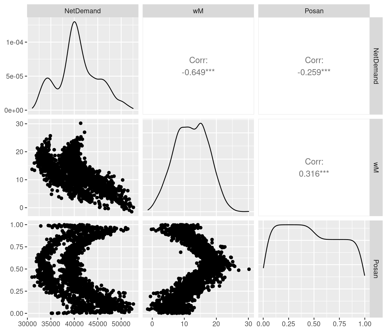

where GGally::ggpairs is the ggplot2 version of graphics::pairs, so the code above is similar to:

pairs( UKload[ , c("NetDemand", "wM", "Posan")] )

We can also remove variables, for instance:

UKload %<>% select(-Date)

removes the Date variable from the data set (notice that we are over-writing UKload by using the assignment pipe %<>%).

Another useful function is filter, which allows you to subset your data using logical conditions, for instance:

coldMondays <- UKload %>% filter(wM < 5 & Dow == "lundi") %T>% 
                          {print(head(.), digits = 2)}

##   NetDemand  wM wM_s95  Posan   Dow   Trend NetDemand.48 Holy Year
## 1     43442 2.1    1.9 0.0068 lundi 1.3e+09        41192    0 2011
## 2     51282 2.9    1.5 0.0836 lundi 1.3e+09        44845    0 2011
## 3     50163 5.0    4.3 0.1411 lundi 1.3e+09        42856    0 2011
## 4     48403 4.5    4.8 0.1603 lundi 1.3e+09        40709    0 2011
## 5     50950 3.9    1.8 0.9658 lundi 1.3e+09        43257    0 2011
## 6     48653 3.7    1.4 0.0424 lundi 1.3e+09        42238    0 2012

Here we are selecting only the Mondays (“Lundi” in French) where the temperature is below 5 degrees Celsius. We are also printing the first and last few rows of the data by exploiting the %T>% pipe (by the way, why do we need the curly brackets {} around print?). Warning: notice that the following would not work:

coldMondays <- UKload %>% filter(wM < 5 && Dow == "lundi") %T>% 
                          {print(head(.), digits = 2)}

## Error in `filter()`:
## ℹ In argument: `wM < 5 && Dow == "lundi"`.
## Caused by error in `wM < 5 && Dow == "lundi"`:
## ! 'length = 2008' in coercion to 'logical(1)'

because we need to use &, which performs elementwise comparisons, not &&, which is typically used for programming control-flow (e.g. in if-else statements). Same for | and ||.

You might also find useful the arrange function, which allows you to sort the rows of the data using one of more variable:

UKload %<>% arrange(Dow, desc(wM)) %T>% 
            {print(head(.), digits = 2)} %T>% 
            {print(tail(.), digits = 2)}

##   NetDemand wM wM_s95 Posan      Dow   Trend NetDemand.48 Holy Year
## 1     34061 25     21  0.63 dimanche 1.3e+09        34780    0 2012
## 2     33680 24     19  0.51 dimanche 1.4e+09        34566    0 2013
## 3     33811 23     20  0.53 dimanche 1.4e+09        34890    0 2013
## 4     33127 23     18  0.40 dimanche 1.3e+09        34191    1 2012
## 5     34237 22     17  0.75 dimanche 1.3e+09        34608    0 2011
## 6     34039 22     17  0.48 dimanche 1.3e+09        35170    0 2011
##      NetDemand    wM wM_s95 Posan      Dow   Trend NetDemand.48 Holy Year
## 2003     49958  1.46  1.032 0.144 vendredi 1.4e+09        49316    0 2013
## 2004     50771  1.42  1.425 0.075 vendredi 1.3e+09        51130    0 2011
## 2005     50054  1.29  1.873 0.056 vendredi 1.3e+09        50110    0 2011
## 2006     51593  1.06  0.548 0.111 vendredi 1.3e+09        51827    0 2012
## 2007     50188  0.32 -1.520 0.092 vendredi 1.3e+09        50334    0 2012
## 2008     52233 -1.43  0.026 0.048 vendredi 1.4e+09        51702    0 2013

Above we are modifying the UKload dataframe by sorting its rows by day of the week (Dow) and by descending temperature (wM) (see, ?desc). More precisely, arrange takes a set of column names or expressions and uses the first to order the rows, the second to break the ties in the first, the third to break the ties in the second and so on. It is slightly annoying that the Dow factor does not have the order we would have liked (e.g. Monday to Sunday), instead it is alphabetical:

levels(UKload$Dow) # sun, thur, mon, tue, wed, sat, frid

## [1] "dimanche" "jeudi"    "lundi"    "mardi"    "mercredi" "samedi"   "vendredi"

This gives us the opportunity to illustrate the mutate function, which allows us to modify one or more variables of the data.frame:

UKload %<>% mutate(Dow = factor(Dow, levels(Dow)[c(3, 4, 5, 2, 7, 6, 1)])) %>% 
            arrange(Dow) %T>% 
            {print(head(.), digits = 2)} %T>% 
            {print(tail(.), digits = 2)}

##   NetDemand wM wM_s95 Posan   Dow   Trend NetDemand.48 Holy Year
## 1     42185 27     22  0.49 lundi 1.3e+09        34039    0 2011
## 2     40404 24     20  0.54 lundi 1.4e+09        33811    0 2013
## 3     40663 23     19  0.55 lundi 1.4e+09        33097    0 2013
## 4     39546 23     19  0.58 lundi 1.3e+09        32422    0 2011
## 5     40259 23     18  0.41 lundi 1.3e+09        33127    1 2012
## 6     40316 22     18  0.51 lundi 1.3e+09        33166    0 2011
##      NetDemand    wM wM_s95 Posan      Dow   Trend NetDemand.48 Holy Year
## 2003     45234  2.19  -0.23 0.116 dimanche 1.3e+09        45395    0 2012
## 2004     43164  2.18   2.13 0.034 dimanche 1.4e+09        43509    0 2013
## 2005     43395  1.97   1.51 0.045 dimanche 1.5e+09        43380    0 2016
## 2006     45359  1.55   0.39 0.097 dimanche 1.3e+09        47236    0 2012
## 2007     45487  0.42   0.59 0.226 dimanche 1.4e+09        45425    0 2013
## 2008     46566 -0.26  -0.13 0.053 dimanche 1.4e+09        46997    0 2013

Above we are mutating the Dow factor variable by rearranging the order of its levels, in fact:

levels(UKload$Dow) # mon, tue, wed, thur, fri, sat, sun

## [1] "lundi"    "mardi"    "mercredi" "jeudi"    "vendredi" "samedi"   "dimanche"

so that the rows of UKload are now in order we want (Monday to Sunday).

Notice that the functions described so far have a similar set of arguments, for instance:

args(arrange)

## function (.data, ..., .by_group = FALSE) 
## NULL

args(select)

## function (.data, ...) 
## NULL

args(mutate)

## function (.data, ...) 
## NULL

Hence, the first argument is always a data.frame and the ... contains a variable number of arguments which determine what needs to be done with the data (e.g. in select(UKload, wM, Posan) both wM and Posan end up in the ...). The fact that the first argument is a data.frame is important, because it makes so that pipes work smoothly with dplyr.

Grouping and summarizing data.frames

The dplyr package offers also some very convenient tools for grouping and summarizing data frames. To illustrate these, let us load a fresh version of our electricity demand data:

data(UKload)

The summarise function allows you to reduce a data frame to a set of scalar variables, for instance:

UKload %>% summarise(maxDem = max(NetDemand), 
                     meanTemp = mean(wM), 
                     nHoly = sum(Holy == "1"))

##   maxDem meanTemp nHoly
## 1  52596 12.20725    56

Above we are reducing the whole data set to a vector containing the maximum electricity demand, the mean temperature and the total number of holidays, calculated across the whole data.frame. Using summarise in this simple way can be handy sometimes, but we could do the same thing quite easily in base R. It is more interesting to use summarise in conjunction group_by, as the following example illustrates.

Recall that the UKload data set contains daily electricity demand observations (NetDemand), representing the total demand in the UK between 11:30am and 12am (minus embedded production, e.g. from solar panels). Now, suppose that we want to model the total demand during a week, using some of the other variables. To do this it is useful to exploit the group_by function, which takes as input a data.frame and groups its rows using one or more variables. For example:

library(lubridate)
UKweek <- UKload %>% mutate(wk = week(Date)) %>% 
                     group_by(Year, wk)
UKweek

## # A tibble: 2,008 × 11
## # Groups:   Year, wk [291]
##    NetDemand    wM wM_s95   Posan Dow           Trend NetDemand.48 Holy   Year
##        <dbl> <dbl>  <dbl>   <dbl> <fct>         <dbl>        <dbl> <fct> <int>
##  1     38353  6.05   5.56 0.00137 samedi   1293879600        38353 1      2011
##  2     41192  2.80   3.23 0.00411 dimanche 1293966000        38353 0      2011
##  3     43442  2.10   1.86 0.00685 lundi    1294052400        41192 0      2011
##  4     50736  3.44   2.31 0.00959 mardi    1294138800        43442 0      2011
##  5     50438  5.96   4.72 0.0123  mercredi 1294225200        50736 0      2011
##  6     50064  4.12   4.59 0.0151  jeudi    1294311600        50438 0      2011
##  7     51698  3.08   2.45 0.0178  vendredi 1294398000        50064 0      2011
##  8     43988  7.08   7.25 0.0205  samedi   1294484400        51698 0      2011
##  9     43340  4.89   3.53 0.0233  dimanche 1294570800        43988 0      2011
## 10     50645  6.33   3.47 0.0260  lundi    1294657200        43340 0      2011
## # ℹ 1,998 more rows
## # ℹ 2 more variables: Date <dttm>, wk <dbl>

Here we are using mutate and lubridate::week to create a new variable, wk \(\in \{1, 2, \dots, 53\}\), indicating the week to which each observation belongs and then we are grouping the data by year and week. As you can see, the output of group_by is not just a data.frame but a tibble, which is a “tidy” version of a data.frame. Without going too much into details, tibbles inherits the data.frame class:

class(UKweek)

## [1] "grouped_df" "tbl_df"     "tbl"        "data.frame"

so we can use them pretty much as if they were just data.frames. Notice that the structure of the UKweek tibble is printed nicely on the console, in fact we can see its size, the class of each variable (e.g. wM is a double <dbl> and Dow is a factor <fct>) and we can also see that it has been grouped by year and week (Groups: Year, wk [1]).

The fact that the UKweek has been grouped by week and year, makes so that if we perform dplyr-based operations to it, these will be applied by group. For instance, here:

UKweek %<>% summarise(TotDemand = sum(NetDemand),
                      tempMax = max(wM), 
                      tempMin = min(wM),
                      Posan = mean(Posan), 
                      nHoly = factor(sum(Holy == "1")))

## `summarise()` has grouped output by 'Year'. You can override using the
## `.groups` argument.

UKweek

## # A tibble: 291 × 7
## # Groups:   Year [6]
##     Year    wk TotDemand tempMax tempMin   Posan nHoly
##    <int> <dbl>     <dbl>   <dbl>   <dbl>   <dbl> <fct>
##  1  2011     1    325923    6.05   2.10  0.00959 1    
##  2  2011     2    332107   12.5    4.89  0.0288  0    
##  3  2011     3    329419   12.2    1.29  0.0479  0    
##  4  2011     4    340075    7.63   1.42  0.0671  0    
##  5  2011     5    339415   11.3    0.968 0.0863  0    
##  6  2011     6    319443   11.5    7.05  0.105   0    
##  7  2011     7    320058    8.85   6.01  0.125   0    
##  8  2011     8    323699   13.0    4.46  0.144   0    
##  9  2011     9    321129    8.28   3.07  0.163   0    
## 10  2011    10    314010   10.8    4.83  0.182   0    
## # ℹ 281 more rows

we are calculating the weekly total demand, max and min temperature, the mean position along the year (Posan) and the total number of holidays (ranging from 0 to 7). Now we have a weekly demand data set but, before starting modelling it, we discard the last two weeks and the first week of the year by doing:

UKweek %<>% filter(wk < 52 & wk > 1)

The reason for this is that the Christmas and New Year period is quite special in terms of electricity demand dynamics, hence we prefer to discard it here.

A simple GAM model for weekly total demand might be \(D_w \sim N(\mu_w, \sigma)\) where \[ \mu_w = \mathbb{E}(D_w) = \psi_{N_w} + f_1(T^{max}_w) + f_2(T^{min}_w) + f_3(\text{Posan}_w), \] \(\psi_{N_t}\) is a parametric effect, whose value depends on the number of holidays taking place during the \(w\)-th week, while \(f_1, f_2\) and \(f_3\) are smooth effects (see a previous section for an intro to GAMs, but a deep understanding of GAMs is unnecessary here, as we just want to illustrate the utility of dplyr in day-to-day modelling). We fit the model as follows:

library(mgcViz)
fit <- gamV(TotDemand ~ nHoly + s(tempMax) + s(tempMin) + s(Posan), data = UKweek)

and we then plot the effects:

print(plot(fit, allTerms = TRUE), pages = 1)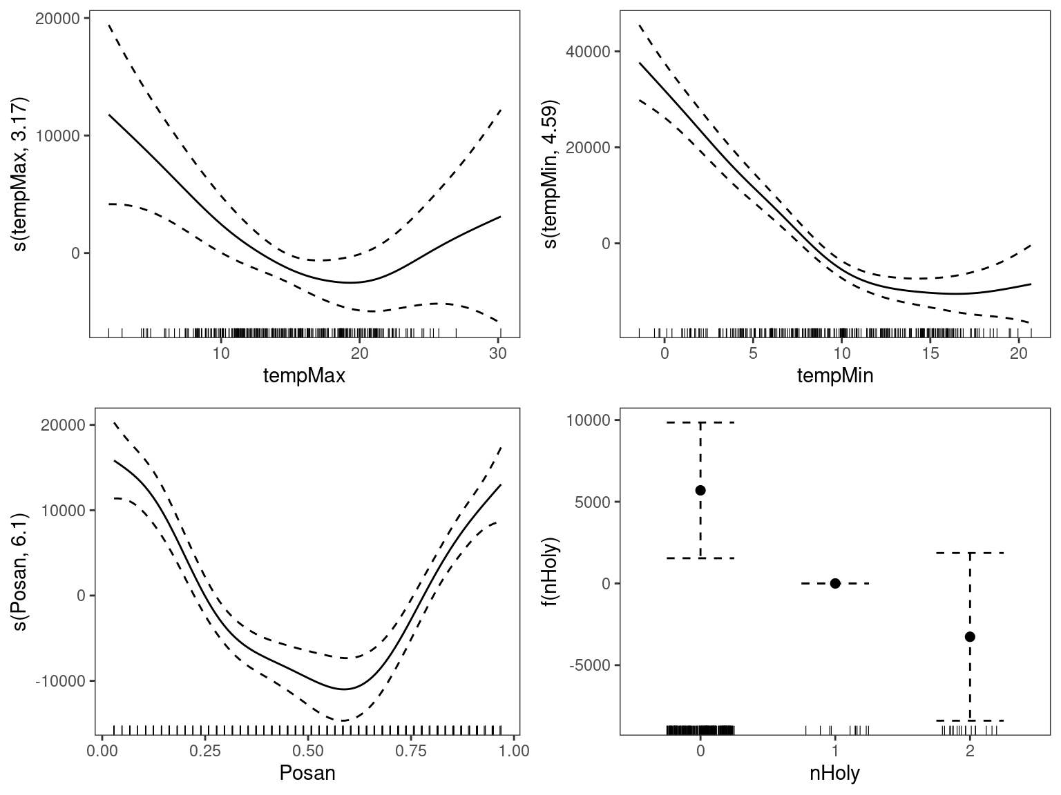

We can see a strong heating effect depending on the minimal weekly temperature, but little cooling effect (recall that this is UK data!). As expected consumption is higher in the winter than in the summer, and weeks containing holidays have a lower total consumption.

This section showed how to use the basic tools provided by dplyr to transform data.frames. To appreciate the practical utility of such tools, you are encouraged to try to transform UKload into UKweek using only the tools provided by base R (that is, without using group_by and summarise). You are also encouraged to issue a pull request including your solutions, as it would be cool to see how base R solutions to this problem look, relative to the dplyr-based solution above.