1. A very short introduction to pipes
Here we introduce the pipe operator, which is provided by the magrittr R package. This introduction is extremely short, and we refer to R for Data Science for details. We start by explaining what pipes are, how they work and then we will give examples of when they are useful.
Pipes basic
The pipe operator %>% is quite simple, but very useful in certain situations. In RStudio, you can use the keyboard shortcut Ctrl + Shift + M to produce %>%. Consider the following code:
x <- seq(0, 2*pi, by = 0.01)
plot(sqrt(abs(cos(x))))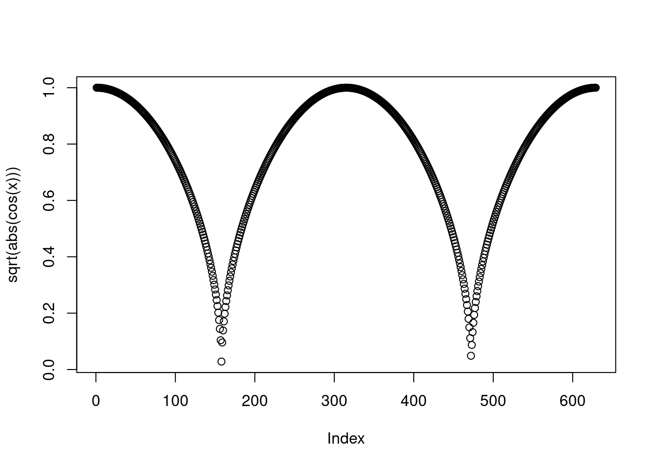 which is plotting \(\sqrt(|\text{cos}(x)|)\). The piped version of this is:
library(magrittr)
x %>% cos %>% abs %>% sqrt %>% plot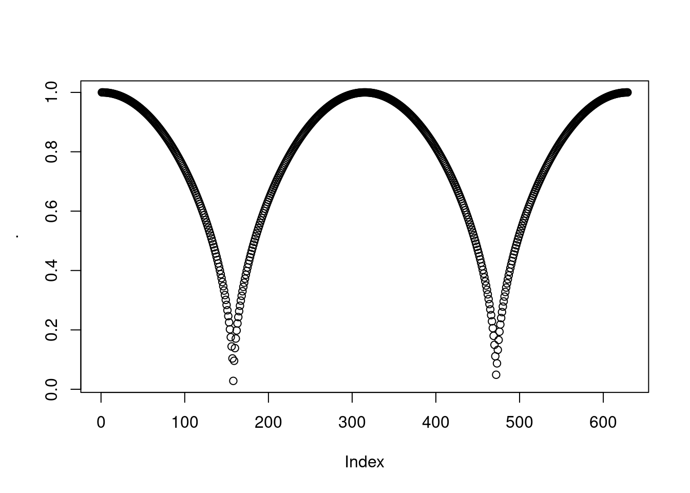 As you can see, the output is the same, with the exception of the y-axis label, which is now “.” (we’ll explain the reason for that in a moment). Now, what is happening? Essentially, the pipe operator is used in expressions of the type
 R_object %>% A_function and it transforms this expression into something equivalent to A_function( R_object ). So the function composition f1(f2(x)) becomes x %>% f2 %>% f1.
To be more precise, the code x %>% cos %>% abs %>% sqrt %>% plot is equivalent to:
 myFun <- function(.){

 . <- cos( . )
 . <- abs( . )
 . <- sqrt( . )
 plot( . )

}

myFun(x)
that is, we are applying a sequence of functions and we are storing the partial results in the “.”. This should explain why
 . appears in the y-axis label.
Now, what do we do if we want to specify some extra arguments, for example as in the code:
plot(x = x, y = sqrt(abs(cos(x))), ylab = "y") ? This is achieved as follows:
x %>% cos %>% abs %>% sqrt %>% plot(x = x, y = ., ylab = "y")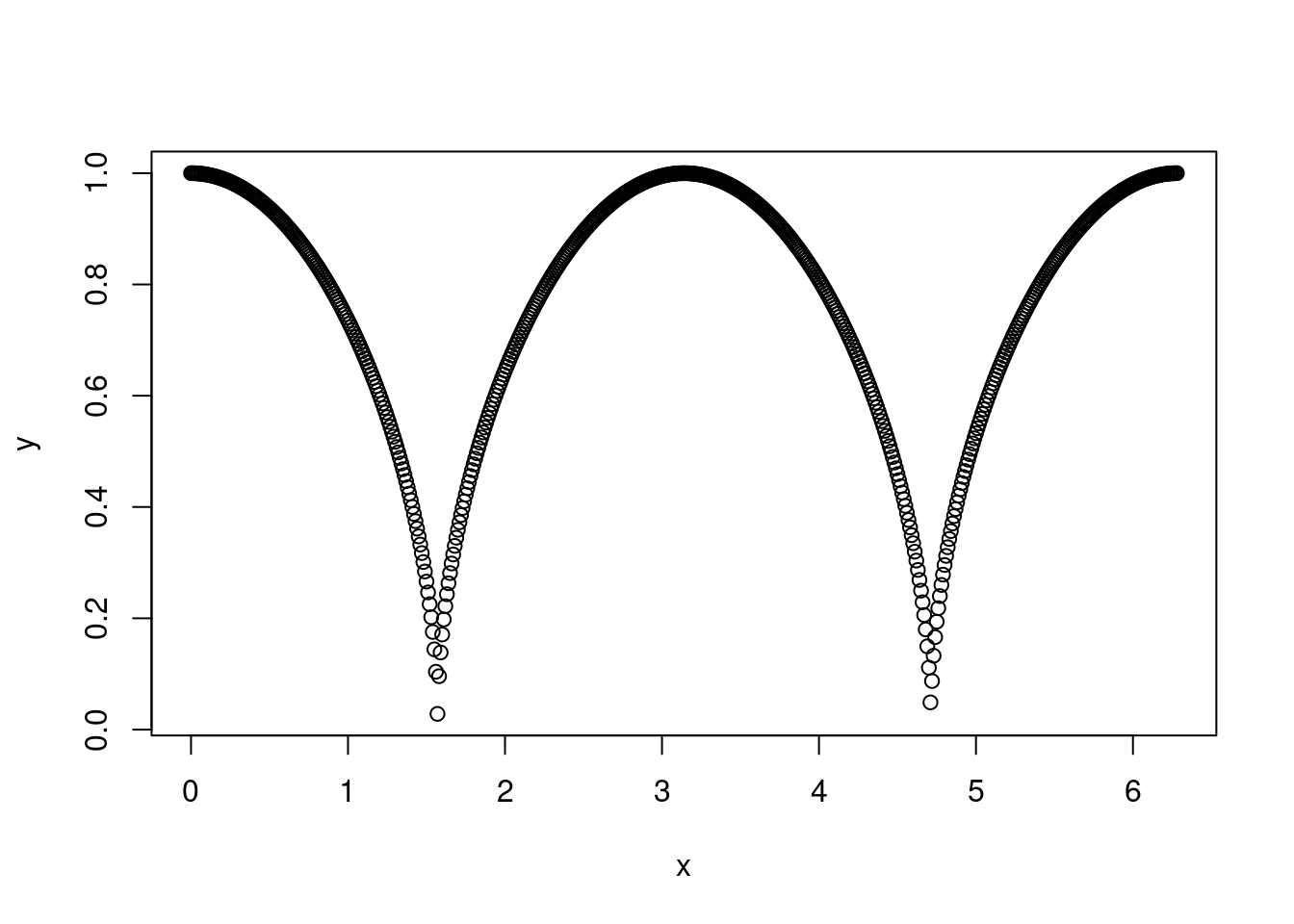 Hence, we use
 . as a placeholder for the argument that is being piped (the lhs of the pipe operator).
WARNING: a clarifications is needed here. By default the placeholder . will be used as the first argument of the function to be applied (here plot()). That is, x %>% plot(ylab = "y") is equivalent to plot(., ylab = "y") where . is equal to x, the lhs of the pipe. This behaviour is overridden if the placeholder appears somewhere on the rhs. For instance y %>% plot(x = x, col = .) is not equivalent to plot(., x = x, col = .) with . == y, but it is the same as plot(x = x, col = y). Hence, if we use the placeholder explicitly on the rhs of the pipe, the placeholder . will not be assigned to the first argument of the rhs function. However, notice that the following does not work:
x %>% plot(x = x, y = . + 1, ylab = "y")
# Error in plot.xy(xy, type, ...) : invalid plot type
Why? Because here the placeholder appears only the nested expression (. + 1) and the above code is equivalent to plot(., x = x, y = . + 1, ylab = "y") with . == x, which leads to an error. Hence, when the placeholder appears only in nested expressions on the rhs of the pipe, the %>% follows the default behaviour consisting of using the . (where . == x here) as the first argument of the rhs function to be applied (plot). To override this behaviour, we must sandwhich the rhs of the pipe using curly {} brackets:
x %>% { plot(x = x, y = . + 1, ylab = "y") } which makes so that the
 . is used only in the function arguments where it appears explicitly.
Having clarified this, we can now show how the . can be used multiple times inside the rhs function, for instance:
3 %>% { matrix(1 : (. * .), ncol = ., nrow = .) }## [,1] [,2] [,3]
## [1,] 1 4 7
## [2,] 2 5 8
## [3,] 3 6 9is equivalent to matrix(1 : (3 * 3), ncol = 3, nrow = 3). Also, we can split up the lhs of the pipe into its elements, for instance:
x <- list(letters[1:6], 2, 3, TRUE)

x %>% { matrix(.[[1]], nrow = .[[2]], ncol = .[[3]], byrow = .[[4]]) }
## [,1] [,2] [,3]
## [1,] "a" "b" "c"
## [2,] "d" "e" "f"which is equivalent to matrix(letters[1:6], nrow = 2, ncol = 3, byrow = TRUE).
When are pipes useful?
Having gone through the introduction to pipes, you might wonder why should you care given that you can obtain the same result using a composition of functions. Indeed, the first example where we plotted \(\sqrt(|\text{cos}(x)|)\) is simple enough for explaining how pipes work, but it is not an example where pipes are useful (doing plot(sqrt(abs(cos(x)))) might be clearer). To motivate pipes, consider the following example:
library(qgam)
data(UKload)
head(UKload)
## NetDemand wM wM_s95 Posan Dow Trend NetDemand.48
## 25 38353 6.046364 5.558800 0.001369941 samedi 1293879600 38353
## 73 41192 2.803969 3.230582 0.004109824 dimanche 1293966000 38353
## 121 43442 2.097259 1.858198 0.006849706 lundi 1294052400 41192
## 169 50736 3.444187 2.310408 0.009589588 mardi 1294138800 43442
## 217 50438 5.958674 4.724961 0.012329471 mercredi 1294225200 50736
## 265 50064 4.124248 4.589470 0.015069353 jeudi 1294311600 50438
## Holy Year Date
## 25 1 2011 2011-01-01 12:00:00
## 73 0 2011 2011-01-02 12:00:00
## 121 0 2011 2011-01-03 12:00:00
## 169 0 2011 2011-01-04 12:00:00
## 217 0 2011 2011-01-05 12:00:00
## 265 0 2011 2011-01-06 12:00:00Here we are loading data on total electricity demand in the UK. Variable NetDemand is the demand, Posan is a cyclical variable indicating the position along the year and Dow is the day of the week (in French!). See ?UKload for an explanation regarding the meaning of the other variables. Now let’s look at the following code:
plot(NetDemand ~ Posan,
transform(
head(
subset(UKload, Dow == "lundi", select = c("NetDemand", "Posan")),
100),
Posan = Posan * 365)
)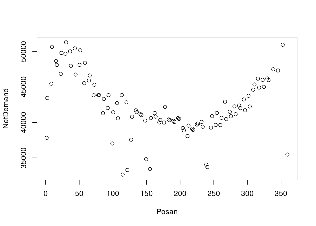 What are we doing here? We are performing the following steps:
subsetselects the Mondays ("lundi") and theNetDemandandPosancolumns;headselects the first 100 rows;transformmakes so thatPosantakes value in \([0, 365]\) rather than \([0, 1]\).plotplotsNetDemandvsPosan.
Now, to understand what is going on here, you need to read the code from the inner-most function call (subset) to the outer-most one (plot). So the code does not clearly express the sequence of operations detailed in the numbered list above. This is an example where pipes lead to much clearer code:
UKload %>%
  subset(Dow == "lundi", select = c("NetDemand", "Posan")) %>%
  head(100) %>%
  transform(Posan = Posan * 365) %>%
  plot(NetDemand ~ Posan, data = .)
In fact, we can understand which operations are being performed by simply going from the top to the bottom line. It is also clear what arguments are being provided to each function. In summary, pipes are useful when you are calling a sequence of functions where the output of one function is going to be the input of the next one.
Advanced piping
Here we briefly mention some more exotic types of pipes.
The assignment pipe %<>%
Consider the following code:
x <- c(5, 1, 7, 9, 3)

x %<>% sort

x
## [1] 1 3 5 7 9What happened? Here the assignment pipe %<>% is a shortcut for x <- x %>% sort. That is, it performs the pipelined operations and then it stores the result in x. Importantly, %<>% can only be the first pipe in a pipeline, so that:
x <- c(5, 1, 7, 9, 3)

x %>% sort %<>% sort(decreasing = TRUE)
generates an error. Instead:
x <- c(5, 1, 7, 9, 3)

x %<>% sort %>% sort(decreasing = TRUE)

x
## [1] 9 7 5 3 1does modify x. Notice that x is in decreasing order, so the output of the last pipe in the pipeline is stored in x.
The tee pipe %T>%
Consider the code:
100 %>%
seq(0, 2*pi, length.out = .) %>%
cos %>%
plot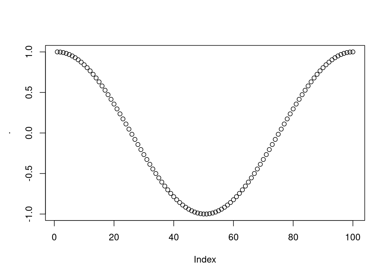 which is plotting the \(\text{cos}(x)\) at 100 values in \([0, 2\pi]\). Now, what if also we want to store the computed values of \(\text{cos}(x)\)? The following would not work:
x <- 100 %>%
  seq(0, 2*pi, length.out = .) %>%
  cos %>%
plotx## NULLIn fact, we are storing in x the output of the final function in the pipe, which is plot (and plot returns NULL). Storing partial results of the pipe requires using the %T>% operator as follows:
x <- 100 %>%
  seq(0, 2*pi, length.out = .) %>%
  cos %T>%
plotx[1:10]## [1] 1.0000000 0.9979867 0.9919548 0.9819287 0.9679487 0.9500711 0.9283679
## [8] 0.9029265 0.8738494 0.8412535This produces the plot (not shown) and returns the output of the call to cos(). The %T>% operator differs from %>% because it returns output of its lhs, rather than of its rhs. As a final example consider:
par(mfrow = c(1, 2))
100 %>%
seq(0, pi, length.out = .) %>%
cos %T>%
plot(ylab = "cos(x)") %>%
acos %>%
plot(ylab = "acos(cos(x))")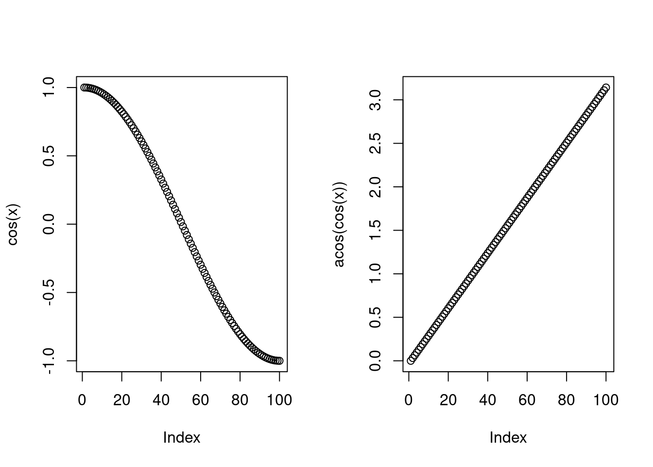 which clarifies that the
 cos %T>% plot section of the pipeline passes the output of cos() to the next section. So the %T>% operator is useful when you want to “keep piping” by skipping the output of one pipeline component. In this specific example we are not interested in the output of plot, which is being called only for its side effects (the plot it draws).
The exposition pipe %$%
This type of pipe is useful when working with named lists and data frames. Consider the example:
UKload %>%
  subset(Year == 2011) %>%
  { cor(.$wM, .$NetDemand) }
## [1] -0.6858647We compute the correlation between electricity demand and temperature in 2011 (see above for explanations regarding why we need the curly brackets here). Now, we can do the same with less code by doing:
UKload %>%
  subset(Year == 2011) %$%
  cor(wM, NetDemand)
## [1] -0.6858647Here the %$% operator makes so that the names of the object on the lhs are available in the function call on the rhs. In base R this would be achieved using the with function:
with(UKload %>% subset(Year == 2011), cor(wM, NetDemand))## [1] -0.6858647